Interpretability by design is usually a conscientious effort. Researchers will think of new architectures or adaptions to existing ones that allow you to understand how they work without additional methods. However, occasionally, we discover something about existing architectures that provide insights into their inner workings.
This latter scenario is how class activation maps (CAMs) were created [2]. Researchers discovered that networks with a specific type of pooling layer, called global average pooling (GAP), were inherently interpretable. By using the weights from this layer, we can learn about how a model is making a classification.
This lesson we will understand:
- How GAP layers work
- How their weights can be used to explain the network
- and how to use them to create CAMs with Python from scratch
We will see that this approach is similar to the method from the lesson on Grad-CAM. In fact, they are mathematically related. In the end, we will discuss this relationship and use it to understand the pros and cons of interpretability by design vs post-hoc methods.
Global Average Pooling (GAP)
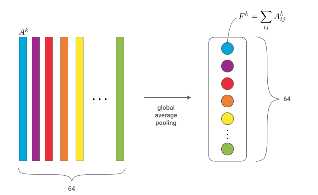
GAP is a dimensionality reduction technique. When included in a neural network, it can be seen as an alternative to pooling methods like max or average pooling. These methods downsample a feature map by calculating a single representative value for a region of the map. In comparison, GAP calculates a single value for the entire feature map.
You can see how GAP does this in Figure 1. The colourful bars represent the feature maps, \(A^k \), in the convolutional neural network. GAP produces one value, \(F^k \), for each map by summing all the elements. In this case, we go from 64 feature maps to 64 values, significantly reducing the dimensionality of the network.
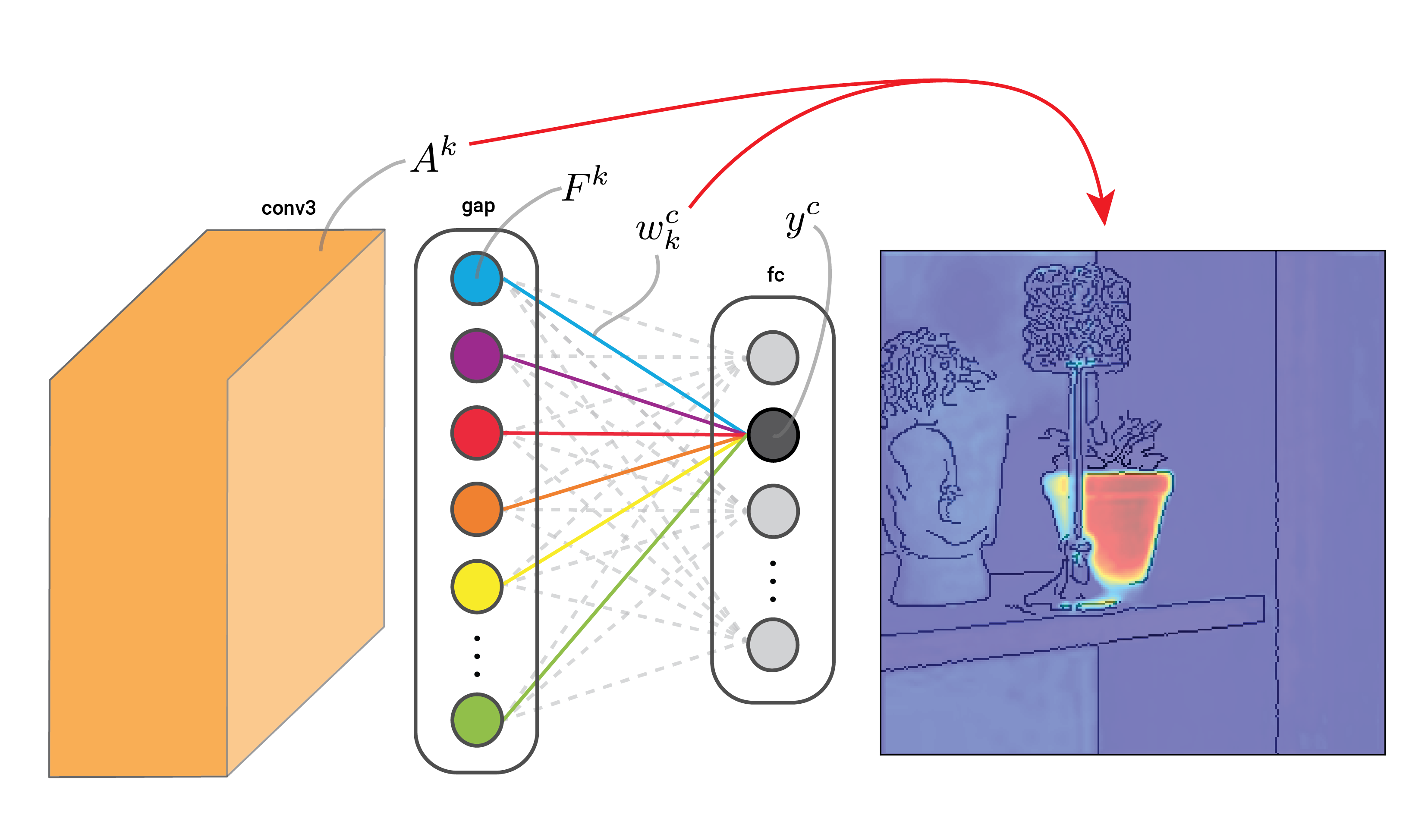
In Figure 2, you can see an example of how a GAP layer can be included in the network. In this case, we have three convolutional layers with an increasing number of feature maps, conv1, conv2 and conv3. The GAP layer comes after conv3. It will have the same number of values, \(F^k \), as there are feature maps, \(A^k \), in conv3. Finally, we have a fully connected layer that connects all output logits, \(y^c\), to the GAP values with weights, \(w^c_k\). The equation below gives the precise formula.
\[
y^c = \sum_k w_k^c F^k + \beta
\]
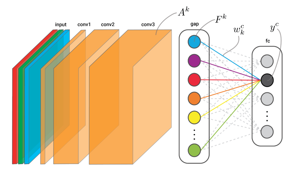
Note that, to create CAMs, the GAP network doesn’t have to look exactly like Figure 2. You could include more convolutional layers, max-pooling layers between the convolutional layers or any other mechanism really. What is important is the final three layers. CAMs require a convolutional layer, followed by GAP and a fully connected layer. To explain why, let’s see how they work.
The theory behind Class Activation Maps (CAMs)
The C in CAM is important. We want to create a saliency map that shows which pixels in the input image have contributed to the logit of the class of interest, \(y^c\). To start we do a forward pass through the network using a given input image. This means all the elements (i.e. feature maps) will be populated. Typically, \(y^c\) will be the largest output logit for this image.
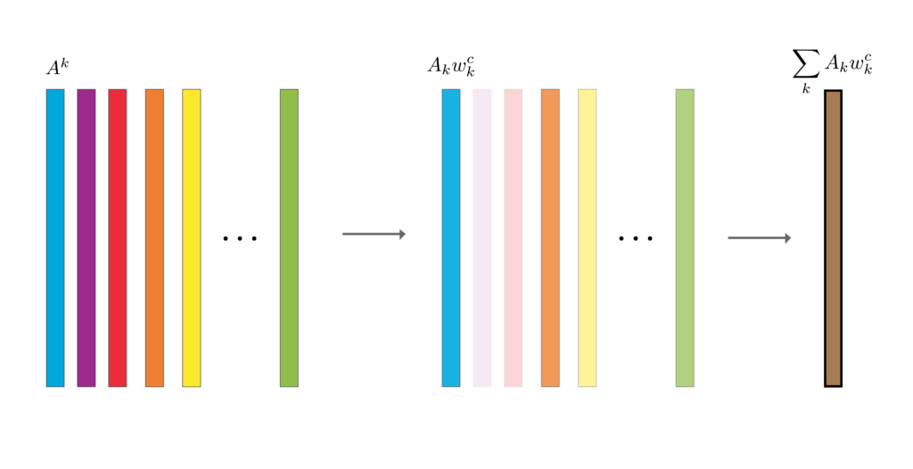
Looking at Figure 3, we weight each feature map in the final convolutional layer, \(A^k\), by the GAP weights for class \(c\), \(w_k^c\). Finally, we do an element-wise summation of weighted feature maps. The result is our CAM. It is a heatmap showing the most important pixels in the input image.
When doing this, keep in mind that the weights are a parameter of the model. Also, we call these GAP weights but they are the weights used in the fully connected layer that produces the output logits. They will be different for each of the classes in the output but they will not change. On the other hand, the feature maps will change depending on the input. The GAP values will also change but these are not used to create the CAM.
In some cases, you will need an additional interpolation step. For our network, this is not necessary as the conv3 layer will have the same height and width as the input. If you have any intermediate pooling layers, you will need to adjust the CAM so it has the same dimensions as the input. Like with Grad-CAM, you can also apply the ReLU activation function to remove any negative values from the CAM.
The steps behind CAMs are intuitive. The feature maps will contain activated elements for all features in the image and not only those that have increased \(y^c\). However, the GAP values, \(F^k\), and their associated feature maps, \(A^k\), that have increased the logit will have larger weights, \(w_k^c\). So, when we weight the feature maps using these, we reduced the influence of irrelevant features on the final CAM.
We discuss similar intuition in more depth in the lesson on Grad-CAM. Later we will see that these two approaches are mathematically related. Specifically, Grad-CAM is a more generalised version of CAM. For now, we will move on to applying CAMs with Python. By coding them from scratch, you may get a better understanding of the theory above.
Class Activation Maps (CAMs) with Python from scratch
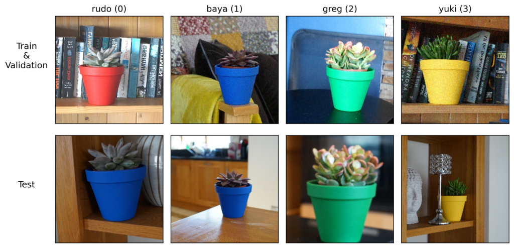
To apply CAMs, we’ll go back to the Pot Plant Dataset (CC BY 4.0). As seen in Figure 4, it is an image classification dataset where we aim to predict the names of 4 different pot plants.
We used this dataset to create Grad-CAM heatmaps. So to avoid repetition, I will gloss over the code used to load the model and dataset. Take a look at that previous lesson if these steps are unclear.
Load model and dataset
We start with our imports. Excluding the grad-cam package, these are the same as the previous lesson.
# Imports
import numpy as np
import matplotlib.pyplot as plt
import cv2
import torch
import glob
from huggingface_hub import hf_hub_download
# Change sys path to import from parent directory
import sys
sys.path.append('../modelling')
from datasets import ImageDataset
from network import CNN
# remove
import importlib
import utils
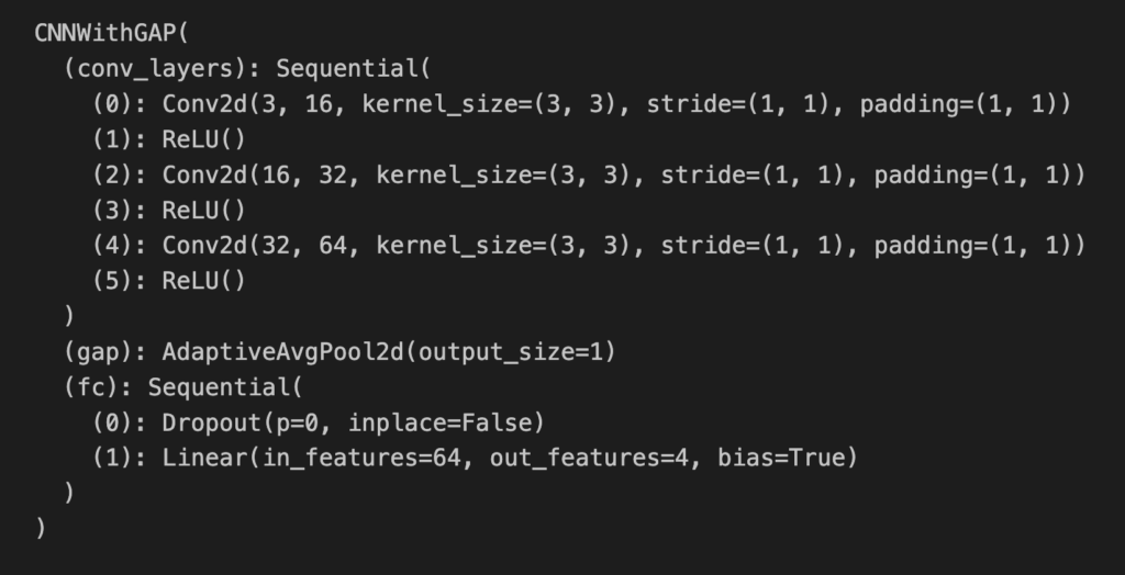
importlib.reload(utils)We load our model. The important difference is the filename (line 3) and model architecture (line 6). We are now using a GAP network. You can see the model summary in Figure 5.
# Download the model directly from Hugging Face Hub
model_path = hf_hub_download(repo_id="a-data-odyssey/XAI-for-CV-models",
                             filename="models/pot_plant_classifier_gap/model.pth")

# Load the model
model = CNNWithGAP()
model.load_state_dict(torch.load(model_path))

# Set the model to evaluation mode
device = torch.device('mps' if torch.backends.mps.is_built()
                      else 'cuda' if torch.cuda.is_available()
                      else 'cpu')
model.to(device)
model.eval()
The summary shows the same architecture as the model we saw in Figure 2. That is three convolutional layers, followed by GAP and a fully connected layer. You can see the last convolution layer, conv_layers[4], has 64 feature maps. After a forward pass, we will use these maps along with the weights from the fully connected layer, fc, to create a CAM.
We create a dataset object for all the images in the test set.
base_path = "../../data/pot_plants/"

plant_names = ['rudo','baya','greg','yuki']
num_classes = len(plant_names)

# Load the data
test_paths = glob.glob(base_path + "/test/*.jpg")
test_data = ImageDataset(test_paths,num_classes)
We load one of the instances from the test set and get a prediction using our GAP network. In Figure 6, you can see that the model has made an incorrect prediction. Now let’s create a CAM to understand what is causing this.
# Get random instance
image, target = test_data.__getitem__(3) # i = 10, 3

# Format input
input = image.unsqueeze(0).to(device)

# Format target
target = torch.argmax(target).item()
target_name = plant_names[target]

# Get the prediction
output = model(input)
pred = torch.argmax(output).item()
pred_name = plant_names[pred]

# Diplay prediction
rgb_image = image.permute(1,2,0).numpy ()
plt.imshow(rgb_image)
plt.title(f"Target: {target_name} ({target})\nPred: {pred_name} ({pred})")
plt.axis('off')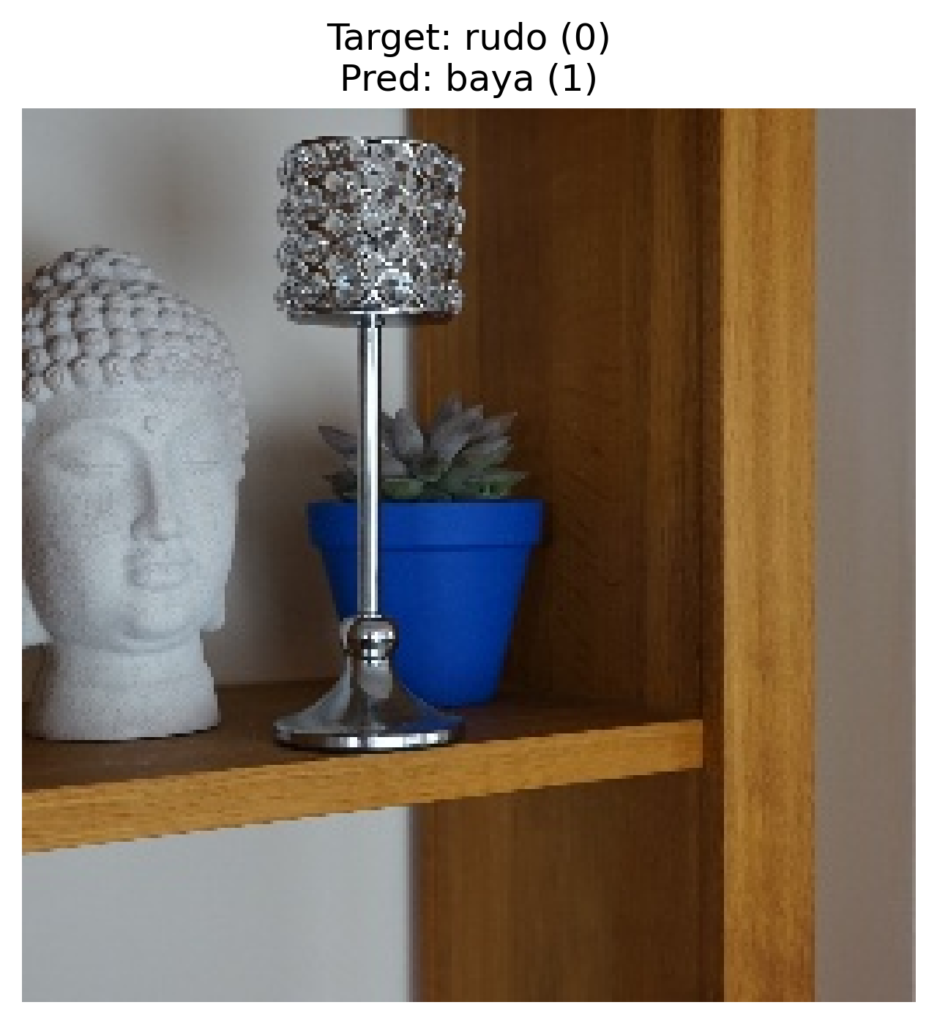
Creating a Class Activation Map (CAM)
We want to create a CAM from the predicted class — baya(1). So, we start by selecting weights from the fully connected layer for this class (line 2). When we output the shape of the weights (line 4) you can see it is a 1D array with 64 elements. In other words, we have 1 weight connecting each of the 64 values in the GAP layer to the logit for class 1.
# Get weights that connect GAP layer to output for class 1
gap_weights = model.fc[1].weight[1]

gap_weights.shape #[1, 64, 256, 256]
As mentioned, the weights will not change depending on the instance. This means we can obtain them before doing a forward pass. This is not true for the feature maps. We must populate their elements using a forward pass with the instance we want to explain.
To do that we start by selecting the final convolutional layer (line 2) and attaching a hook to it (lines 7-10). When we pass the instance into the model (line 13), the hook will append populated feature maps from the convolutional layer to the feature_maps list (line 5). Outputting the shape (line 18), gives us [1, 64, 256, 256]. So, we have a batch size of 1 and 64 feature maps. Each feature map has 256×256 elements, the same as the input dimensions.
# Get final conv layer
final_conv_layer = model.conv_layers[-2]

# Hook to get the feature map from the last conv layer
feature_maps = []

def hook_fn(module, input, output):
    feature_maps.append(output)

hook_handle = final_conv_layer.register_forward_hook(hook_fn)

# Forward pass to get feature maps
model(input)

# Remove the hook
hook_handle.remove()

feature_maps[0].shape
With the feature maps and the weights, we can create our CAM. We start by formatting these as numpy arrays (lines 2-3). We then do element-wise summation. Here every feature map is weighted by the association GAP weight for the class of interest (lines 6-8).
# Extract feature maps and GAP weights
feature_maps = feature_maps[0].squeeze(0).detach().cpu().numpy()  # Shape: [C, H, W]
gap_weights = gap_weights.detach().cpu().numpy()  # Shape: [C]

# Compute the CAM
cam = np.zeros(feature_maps.shape[1:], dtype=np.float32)  # Shape: [H, W]
for i, w in enumerate(gap_weights):
    cam += w * feature_maps[i]
Finally, we apply the ReLU function (line 2) and normalise the CAM using min-max scaling (lines 5-6). This ensures all the values are between 0 and 1.
# ReLU on CAM (optional for better visualization)
cam = np.maximum(cam, 0)
# Normalize CAM for visualization
cam = cam - np.min(cam)
cam = cam / np.max(cam)We then display the CAM (lines 2-4) and you can see the output in Figure 7. Just like before, we can see the model is using the pixels of the pot to make predictions.
# Output class activation map
plt.imshow(cam, cmap="jet", alpha=0.5)
plt.title("Class Activation Map")
plt.axis("off")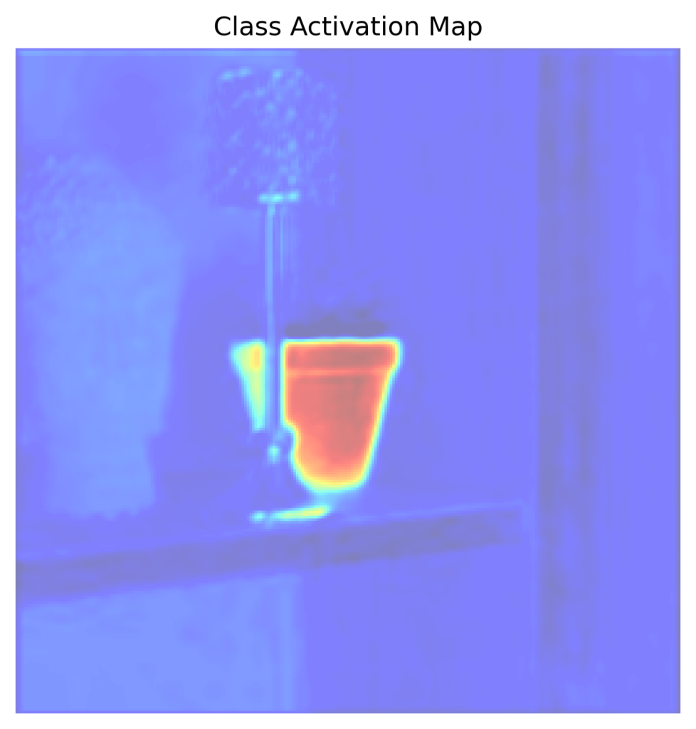
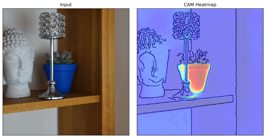
It is also possible to use the functions we used for Grad-CAM, to plot a clearer version of the heatmap. You can see this in Figure 8. You may notice that this output looks very similar to the one we created with Grad-CAM. This is not a coincidence. We’ll discuss this relationship at the end of this lesson.
To end the Python section, we have the generate_cam function. It contains all the code we discussed above.
import torch
import numpy as np
import matplotlib.pyplot as plt
from torchvision.transforms import ToPILImage

# Function to generate CAM
def generate_cam(model, input_image, class_idx):
    """
    Generate Class Activation Map (CAM) for a given input image and class index.

    Args:
    - model (nn.Module): The trained CNN model with GAP.
    - input_image (torch.Tensor): Input image tensor of shape [1, C, H, W].
    - class_idx (int): Index of the class for which CAM is to be generated.

    Returns:
    - cam (np.array): The generated CAM of shape [H, W].
    """
    # Get the final convolutional layer and the GAP weights
    final_conv_layer = model.conv_layers[-1]  # Last convolutional layer
    gap_weights = model.fc[1].weight[class_idx]  # Weights for the class in GAP layer

    # Hook to get the feature map from the last conv layer
    feature_maps = []

    def hook_fn(module, input, output):
        feature_maps.append(output)

    hook_handle = final_conv_layer.register_forward_hook(hook_fn)

    # Forward pass to get feature maps
    model(input_image)

    # Remove the hook
    hook_handle.remove()

    # Extract feature maps and GAP weights
    feature_maps = feature_maps[0].squeeze(0).detach().cpu().numpy()  # Shape: [C, H, W]
    gap_weights = gap_weights.detach().cpu().numpy()  # Shape: [C]

    # Compute the CAM
    cam = np.zeros(feature_maps.shape[1:], dtype=np.float32)  # Shape: [H, W]
    for i, w in enumerate(gap_weights):
        cam += w * feature_maps[i]

    # ReLU on CAM (optional for better visualization)
    cam = np.maximum(cam, 0)

    # Normalize CAM for visualization
    cam = cam - np.min(cam)
    cam = cam / np.max(cam)

    return cam
Relationship between Class Activation Maps (CAMs) and Grad-CAM
CAMs were originally developed for GAP networks. However, since then the term has come to refer to a collection of methods. They all create saliency maps by weighting the feature maps from a convolutional layer by how important they are to the class of interest.
As we saw, the original CAM uses the weights that connect the GAP values to the logit for the class in the output layer [2]. In a previous lesson, we saw Grad-CAM uses the average gradient of the logits w.r.t to the elements in the feature maps [1]. Due to these similarities, we would expect the approaches to create similar outputs. In fact, this relationship goes deeper than that.
As shown in the Grad-CAM paper, Grad-CAM is a generalised version of CAM. In other words, if you applied Grad-CAM to a GAP network you would obtain the same saliency maps as if you had used CAMs. You can see this in Figure 9. Here we have applied both CAM and Grad-CAM to the GAP network above.
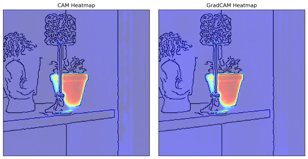
We won’t go over the full proof of this but the intuition is clear. Consider the logits from the GAP network given by the equation below. Remember \(F^k\) is a function of \(A^k\). With Grad-CAM, we would take the derivative of \(y^c\) w.r.t. to the feature maps \(A^k\). Doing this the only value remaining would be \(w_k^c\). In other words, the gradient weights when applying Grad-CAM to a GAP network are the same as the weights used by CAM.
\[
y^c = \sum_k w_k^c F^k + \beta
\]
This relationship highlights the important trade-off between post-hoc methods and interpretability by design (IBD). For IBD methods, we are using the model’s architecture to explain its predictions. This means explanations can be more truthful. However, like how we can only apply CAMs to GAP networks, the downside of IBD is it restricts us to certain types of architectures.
Post hoc methods may provide a low level of interpretability but the flexibility in architecture choice may improve performance. In this case, as the outputs are the same, there is no longer any need to use CAM. However, not all IBD methods will have this problem. Some will provide unique information that cannot be generalised by post-hoc methods. Still, we must keep in mind that using these methods can limit performance.
This is why in practice IBD approaches are usually used for data exploration. That is we want to use neural networks to learn about relationships in our dataset. Our goal is not to maximise performance but to generate new knowledge. This is something we explore in the final lesson on prototype layers.
I hope you enjoyed this article! See the course page for more XAI courses. You can also find me on Bluesky | Threads | YouTube | Medium
Datasets
Conor O’Sullivan (2024). Pot Plant Dataset. (CC BY 4.0) https://www.kaggle.com/datasets/conorsully1/pot-plants
References
[1] Ramprasaath R Selvaraju, Michael Cogswell, Abhishek Das, Ramakrishna Vedantam, Devi Parikh, and Dhruv Batra. Grad-cam: Visual explanations from deep networks via gradient-based localization. In Proceedings of the IEEE international conference on computer vision, pages 618–626, 2017.
[2] Bolei Zhou, Aditya Khosla, Agata Lapedriza, Aude Oliva, and Antonio Torralba. Learning deep features for discriminative localization. In Proceedings of the IEEE conference on computer vision and pattern recognition, pages 2921–2929, 2016.
Get the paid version of the course. This will give you access to the course eBook, certificate and all the videos ad free.