An X-ray AI system displays the result—there is a tumour.
Thankfully, it is benign. However, the doctor is hesitant to give this diagnosis directly to the patient. She doesn’t know where in the brain the tumour is and, to be honest, she doesn’t fully trust the AI system.
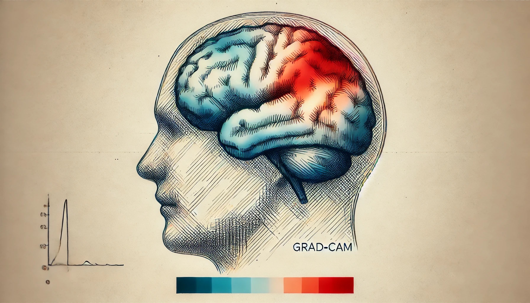
This is where Grad-CAM comes in [3]. It is an explainable AI (XAI) method that can tell the doctor which part of the X-ray image was used to make the classification. It could potentially point out the exact collection of cells that make up the benign tumour.
In general, Grad-CAM is used to explain convolutional neural networks (CNNs). It does this by highlighting the pixels/regions in an image that are important for a given classification. This is known as a heatmap. Due to its speed, reliability and flexibility, Grad-CAM has become the go-to method for creating these.
So, in this lesson, we will:
- Explain the steps taken by the Grad-CAM algorithm to produce heatmaps
- Give the intuition for the method and other CAM approaches
- Discuss its advantages and limitations
- Apply it using Python, PyTorch and the pytorch-grad-cam package.
You may also enjoy this video on the topic. There is another one in the Python section of the lesson. And, if you want to learn more about XAI, check out the courses below 🙂
How the Grad-CAM algorithm works
Grad-CAM produces heatmaps also known as Class Activation Maps (CAMs). These show which parts of an input image are used to classify that image as a particular class. It does this by weighting feature maps in a model’s convolutional layers using the class’s gradients. Using both visualisations and equations, we’ll walk step by step through how these heatmaps are created.
We start with the trained CNN in Figure 1. This one is used to classify an image as a dog or cat. As we pass an input image through the various layers, we reduce the height and width and increase the number of channels. In a convolutional layer, we refer to the channels as feature maps.
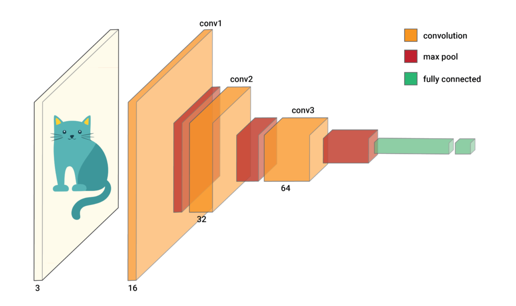
When we do a forward pass through the network with the input image, all the elements of the feature maps will be populated. We will also have logits for each of our classes. For now, we’ll focus on the highest logit, \(y^c\). In other words, the one for the predicted class. To be clear, \(c\) represents an arbitrary class and not necessarily the cat class.
Now, let’s zoom in on the last convolutional layer, conv3. In Figure 2, we can see we have 64 feature maps. To create a GradCAM heatmap, we first weight each feature map so each element has the same weighting. We then do element-wise summation to produce one matrix of elements. We call this the weighted feature map.
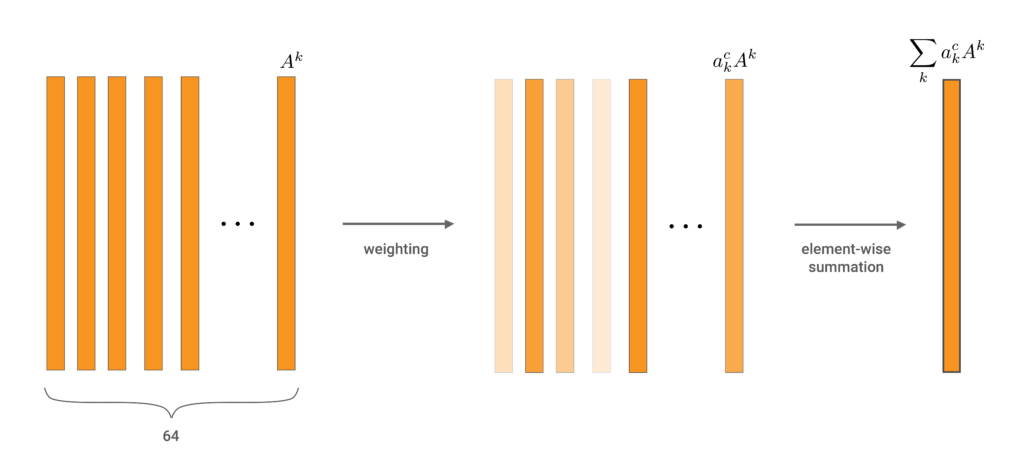
The equation below gives the generalised formula for the weighted feature map. \(a_k^c\) is the weight we apply to feature map \(k\). All CAMs follow this procedure using different approaches to calculating the weights. For gradCAM, they are based on the gradients of the logit for class \(c\).
\[
\sum_{k} a_k^c A^k
\]
To understand how to calculate \(a_k^c\), let’s take a closer look at one of the feature maps. As seen in the equation below, every feature map is a matrix of elements. The dimension (m,n) will depend on how the previous layers have been pooled. \(A_{ij}^k\) is the value for an arbitrary element in the feature map.
\[
A^k = \begin{bmatrix}
A^k_{11} & A^k_{12} & \cdots & A^k_{1n} \\
A^k_{21} & A^k_{22} & \cdots & A^k_{2n} \\
\vdots & \vdots & \ddots & \vdots \\
A^k_{m1} & A^k_{m2} & \cdots & A^k_{mn}
\end{bmatrix}
= \left\{ A^k_{ij} \mid 1 \leq i \leq m, \, 1 \leq j \leq n \right\}
\]
Using backpropagation, we can find \(\frac{\partial y^c}{\partial A_{ij}^k}\). This is the derivative of the logit, \(y^c\), w.r.t. an element of a feature map. This gradient will tell us how much the logit changes with small changes in the element. In other words, larger gradients indicate that the element is more important to the logit.
Looking at the equation below, we can understand how important the entire feature map is by taking the average of all gradients. This is similar to the process of Global Average Pooling (GAP). Except we are now summing derivatives and not the original element values. Ultimately, this GAP gives us the weight for the given feature map.
\[
a_k^c = \frac{1}{Z} \sum_{i} \sum_{j} \frac{\partial y^c}{\partial A_{ij}^k}
\]
So we multiply each feature map by its weight and do element-wise summation. Then only two more steps are needed to create the heatmap. These can be seen in Figure 3. Firstly, some of the elements of the weighted feature map will have negative values. However, we are only interested in the elements that have increased the logit of the predicted class. So, we use the ReLU activation function to ensure all negative elements will have a value of zero.
This gives us a coarse heatmap. The problem is this will have the same dimension (m,n) as the feature maps in conv3. So, the last step is to increase the dimensions so they are the same as the input image. This is done by upsampling using interpolation techniques.
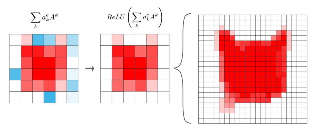
In the end, we can summarise the Grad-CAM heatmap using the equation below. It is obtained by applying the ReLU activation function to the weighted sum of the feature maps in the final convolutional layer. Where the weight for each feature map is the average gradient of the logit for the predicted class w.r.t. to the elements in the feature map.
\[
L_{Grad-CAM}^c = ReLU\left( \sum_{k} a_k^c A^k \right)
\]
For our problem, this will show us which pixels in the input image are used to classify the image as a cat. When applying this method more generally there are a few considerations:
- We’ve talked about applying it to the final convolutional layer, conv3. However, the same process can be applied to any convolutional layer or even a combination of layers. The final layer is usually used as it generally captures the most detailed semantic information.
- We can apply this method to any class and not necessarily the one with the highest logit. This can be useful when trying to understand incorrect predictions.
So hopefully the process behind Grad-CAM heatmaps is clear. However, it doesn’t explain a crucial aspect — why do they work? Let’s move on to understanding the intuition behind this method. That is how it can reliably identify pixels that are relevant for a classification.
The intuition behind Grad-CAM and other CAMs
Grad-CAM was inspired by another method called Class Activation Maps (CAMs) [5]. However, since then the term has come to refer to a collection of methods. They all create heatmaps by weighting the feature maps from a convolutional layer by how important they are to the class of interest.
The original CAM, which we discuss in a future lesson, was used to explain networks with a Global Average Pooling (GAP) layer. It uses the weights that connect the GAP values and the logit for the class in the output layer. Another adaption, ablation-cam, calculates the weights by deactivating entire feature maps and measuring the change in the logit [2]. As we saw, Grad-CAM uses the average gradient of the logit w.r.t to the elements in the feature maps.
All of the methods have been shown to produce heatmaps that reliably explain how the model is making a classification. They work due to the nature of the convolutional layers. These layers, especially the final layers, capture both important features and their spatial information. So, when we do a forward pass the elements for these features, in their location in the input, will be activated.
The problem is that often features that are not relevant to the class of interest will also be activated. This is because other classes or features related to other classes can be in the input. For example, in Figure 4, you can see the first feature map includes elements for the human’s face. If we simply summed all feature maps we would include these irrelevant elements.
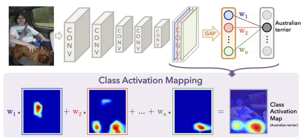
This is why all CAM methods weight the feature maps using some method that captures their importance to the class. By doing so, the heatmap will only give the locations of features that have a significant effect on the predicted logit for that class. The next question is, if all CAM methods do this, then why choose Grad-CAM?
The advantages and limitations of Grad-CAM
The first advantage of Grad-CAM is that it can be applied to any CNN. In comparison, CAMs can only be applied to GAP networks. This means Grad-CAM gives us more flexibility when it comes to architecture selection. Other permutation methods like ablation-cam also have this property.
The advantage of Grad-CAM over permutation methods is that it is not as computationally expensive. We only need to do one forward pass and obtain the gradients for the logit. With ablation cam, we need to do multiple forward passes every time we deactivate a feature map. Other permutation methods like SHAP are even more expensive.
Still, Grad-CAM has its limitations. For some applications, we want detailed explanations for a prediction. We may want to know that the spots on a leopard or the colour of a stop sign have led to a classification. Unfortunately, Grad-CAM can only show that the pixels within a certain region are contributing to the prediction. In a future lesson, we will see how to address this weakness by combining Grad-CAM and guided backpropagation.
Another limitation is that, although Grad-CAM can be applied to many architectures, it is not model agnostic. It has been designed to explain CNNs used for classification tasks. The method can be adapted for regression tasks and there are even adaptions for image segmentation [4]. However, these adaptations will not be the same as the process we have discussed above. They also cannot be applied to transformer-based architectures.
In general, we must consider that all CAMs provide approximations for how a network works. Sometimes these approximations can be wrong or misleading. Through user studies, Grad-CAM has been shown to provide intuitive explanations for predictions [3]. However, it has also been shown that there are networks or instances where the method doesn’t work well [1]. It is important to keep this in mind when applying the method.
Applying Grad-CAM with Python
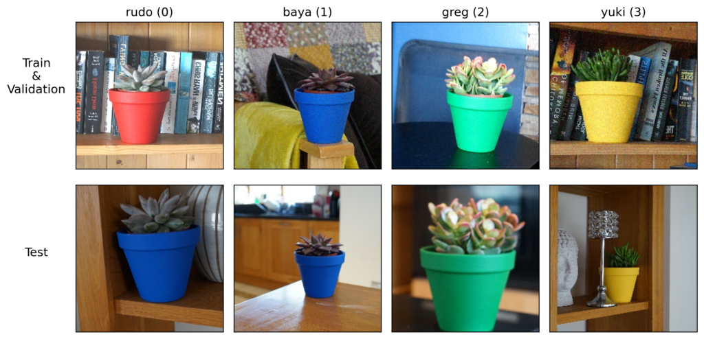
To apply Grad-CAM, we will use the pytorch-grad-cam implementation and we will apply it to the Pot Plant Dataset (CC BY 4.0). This is an image classification dataset where we aim to predict the names of 4 different pot plants.
When we introduced this dataset in a previous lesson, we saw some peculiar behaviour. Looking at Figure 5, we achieved 94% accuracy on the validation set but only 70% on the test set. This decrease in accuracy comes from Rudo being misclassified as Baya.
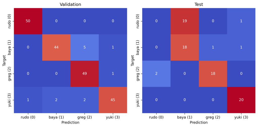
We hypothesised that this had something to do with the pots. During the data collection process, Rudo’s pot was dropped and broken. It seems as though replacing the red pot has confused the model. Let’s use Grad-CAM to see if this is true.
We start with our imports. We’ll load our classification model from hugging face (line 9). We have the imports related to Grad-CAM (lines 11-13). In the src directory there is a folder called modelling. We navigate to this folder (line 16) and load the ImageDataset class from datasets.py (line 19) and the CNN class from network.py (line 20). These are the same classes used to train the model.
# Imports
import numpy as np
import matplotlib.pyplot as plt

import cv2
import torch

import glob
from huggingface_hub import hf_hub_download

from pytorch_grad_cam import GradCAM
from pytorch_grad_cam.utils.model_targets import ClassifierOutputTarget
from pytorch_grad_cam.utils.image import show_cam_on_image

#change sys path to import from parent directory
import sys
sys.path.append('../modelling')

from datasets import ImageDataset
from network import CNN
Load model and dataset
We load our model from the Hugging Face repo (lines 2-7). We then move this model to a GPU (lines 10-13) and set it to evaluation mode (line 14).
# Download the model directly from Hugging Face Hub
model_path = hf_hub_download(repo_id="a-data-odyssey/XAI-for-CV-models",
filename="models/pot_plant_classifier/model.pth")
# Load the model
model = CNN()
model.load_state_dict(torch.load(model_path))
# Set the model to evaluation mode
device = torch.device('mps' if torch.backends.mps.is_built()
else 'cuda' if torch.cuda.is_available()
else 'cpu')
model.to(device)
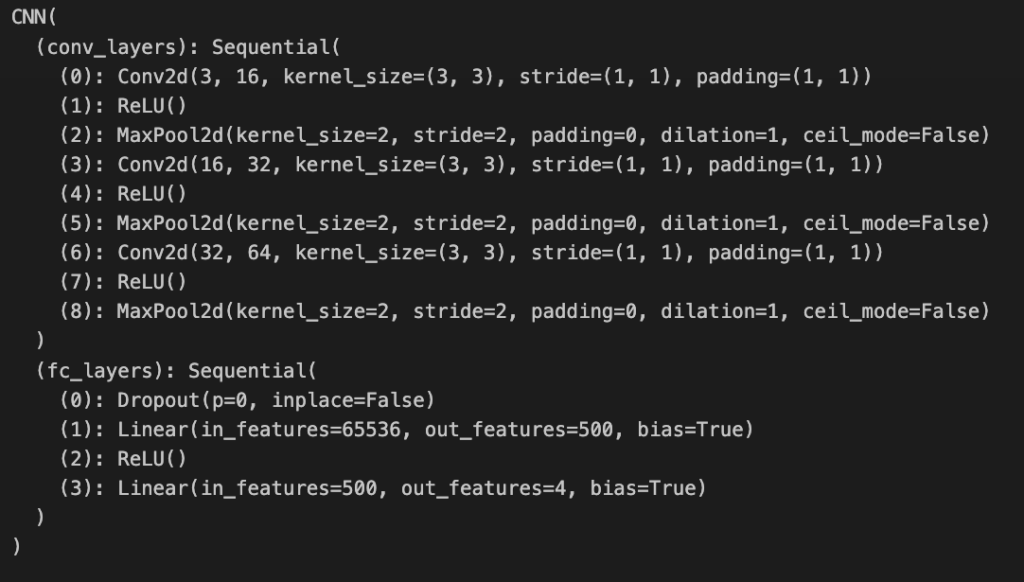
model.eval() You can see the model summary in Figure 7. It has the same architecture as the model we saw in Figure 1. That is three convolutional layers. This summary is important as we must select the layer(s) for which we will create heatmaps. For example, model.conv_layers[6] would select conv3.
We load the paths for the images in the Pot Plant test set (line 7). We then pass these paths into the ImageDataset class to make a dataset object (line 8). This allows us to load the data in the correct format for input into the model. Importantly, we use the correct number of classes. In this case, we have 4 different classes (i.e. plant names) (lines 3-4).
base_path = "../../data/pot_plants/"

plant_names = ['rudo','baya','greg','yuki']
num_classes = len(plant_names)

# Load the data
test_paths = glob.glob(base_path + "/test/*.jpg")
test_data = ImageDataset(test_paths,num_classes)
We load one of the instances from the test set (line 2). The target will be returned as an array of 4 elements. For example, [1,0,0,0] means we have an image of the first plant—Rudo. We format the target to get the class number instead (line 4) and the plant name (line 5).
# Get random instance
image, target = test_data.__getitem__(3)
# Format target
target = torch.argmax(target).item()
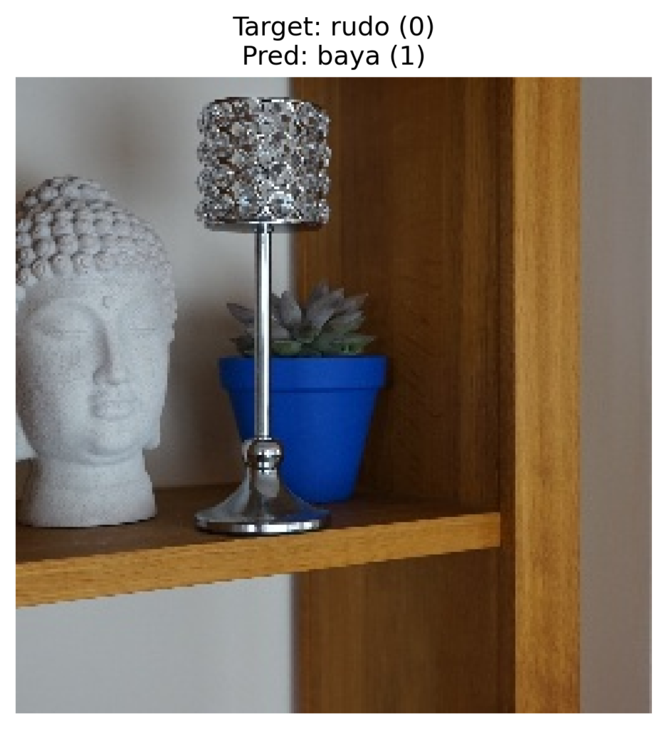
target_name = plant_names[target]We pass the image as input into our model (lines 2-3). Now the output will be a list of 4 logits. Our predicted class will be the position of the highest logit (line 4). Finally, we display the input image, target and predicted class (lines 8-11). You can see the output in Figure 8.
# Get prediction
input = image.unsqueeze(0).to(device)
output = model(input)
pred = torch.argmax(output).item()
pred_name = plant_names[pred]

# Diplay prediction
rgb_image = image.permute(1,2,0).numpy ()
plt.imshow(rgb_image)
plt.title(f"Target: {target_name} ({target})\nPred: {pred_name} ({pred})")
plt.axis('off')
You can have an image of Rudo (0). Keep in mind this is from the test set. We had to change the plant’s pot from red to the blue one you see here. As mentioned, we strongly suspect that this is causing problems. We can see that the predicted class is Baya (1) which had a blue pot in the training set. Let’s see if GradCAM can provide some more evidence.
Visualization Functions
To start, we have a few functions that will help visualise our Grad-CAM heatmaps. The first returns an edge map based on an input image. In Figure 9, you can see the result of this function. It provides the outline/ edges of objects in the image.
def get_canny_edge(img,threshold1=30,threshold2=80):

    """
    Function to get the canny edge of an image
    """

    # Gray scale the image
    gray = cv2.cvtColor(img, cv2.COLOR_RGB2GRAY)
    gray = gray*255
    gray = gray.astype(np.uint8)

    # Gaussian blur
    gray = cv2.GaussianBlur(gray, (5, 5), 0)

    # Get the edge
    edge = 255- cv2.Canny(gray,threshold1, threshold2)
    edge = np.stack([edge]*3,axis=-1)/255

    return edge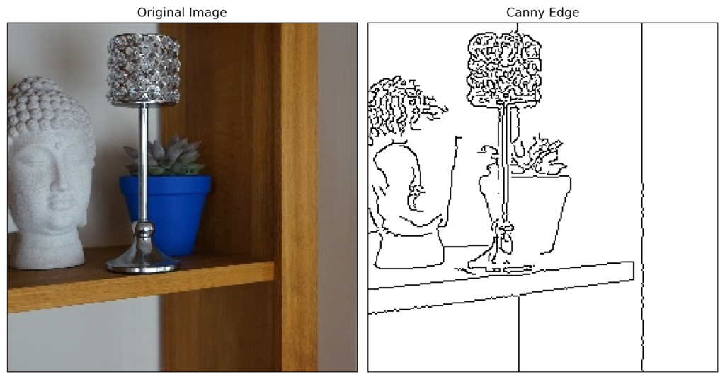
The second function will display the original image and the Grad-CAM heatmap. In the next section, we will see how the visualization is created. In our case, we will plot the grad-CAM heatmaps on top of the edge maps created with the above functions. We do this as it removes any background colour from the input image providing a clearer heatmap.
def plot_gradcam(rgb_image, visulaization,title='Input'):

    """Display the original image and the GradCAM heatmap"""

    fig, ax = plt.subplots(1,2,figsize=(10,5))

    ax[0].imshow(rgb_image)
    ax[0].set_title(title)

    ax[1].imshow(visulaization)
    ax[1].set_title("GradCAM Heatmap")

    for a in ax:
        a.set_xticks([])
        a.set_yticks([])
GradCAM heatmaps
Finally, we can move on to creating and displaying our Grad-CAM heatmaps. We’ll explore different options in terms of the layers and classes we want to explain.
Predicted class and last layer
Typically, with Grad-CAM we focus on the class that had the highest predicted logit. This will provide a heatmap of the important regions for that class. As we saw for our instance in Figure 8, this can be different from the target class. We also tend to focus on the last convolutional layer in the network.
We define both of these aspects in the code below. Both the classes (line 2) and layers (line 3) must be lists. ClassifierOutputTarget is a helper class used in the Grad-CAM library to specify the output class. We have passed a value of 1 as this is the predicted class. We get the last convolutional layer (line 3) from the model output in Figure 7.
# Define the target layer and target class
classes = [ClassifierOutputTarget(1)]
layers = [model.conv_layers[6]]
Next, we create the cam object using our model and layers (line 2). We then use this object to create a heatmap for our instance and desired class (line 3). We must unsqueeze the image as the tensor has a dimension for batch size.
# Get the GradCAM heatmap
cam = GradCAM(model=model, target_layers=layers)
heatmap = cam(input_tensor=image.unsqueeze(0), targets=classes)
The shape of the resulting heatmap is (1,256,256). These are the same dimensions as our input tensor. Ignoring the batch dimension, we now have a matrix where each value gives the importance of the pixels in our input image to the prediction.
print(heatmap.shape)We can see this when we visualise the heatmap. We can display it as an image (line 2). In Figure 10, you can see there is an important region. Let’s use some of the Grad-CAM helper functions to get a clearer picture.
# Display heatmap
plt.imshow(heatmap[0])
plt.axis('off')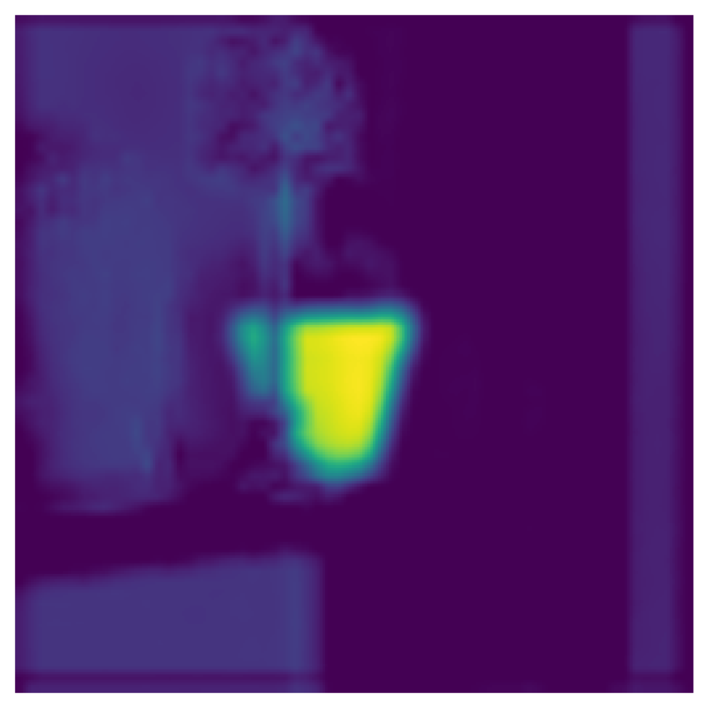
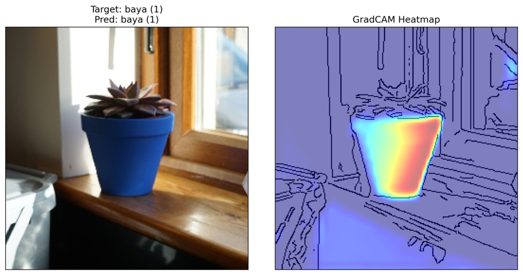
We create an edge map from our input image (line 2). We then use the show_cam_on_image helper function to plot the heatmap on top of the edge map (line 3). By setting, use_rgb = True, the important regions will be red and the least important regions will be blue. Finally, we use our plot_gradcam function to display the input image and visualisation side by side. You can see the result in Figure 11.
# Plot the heatmap
edge = get_canny_edge(rgb_image)
visulaization = show_cam_on_image(edge, heatmap[0], use_rgb=True)

plot_gradcam(rgb_image, visulaization)
Clearly, the model is using the pixels from the pot to make the prediction. This confirms our suspicion. By taking pictures of the plants in only one pot we have introduced bias. The model has learned to classify the plants based on their pots and not their inherent characteristics. As a result, when we moved Rudo to a new pot in the test set the model became “confused”. In short, we have built a pot detector and not a plant detector.
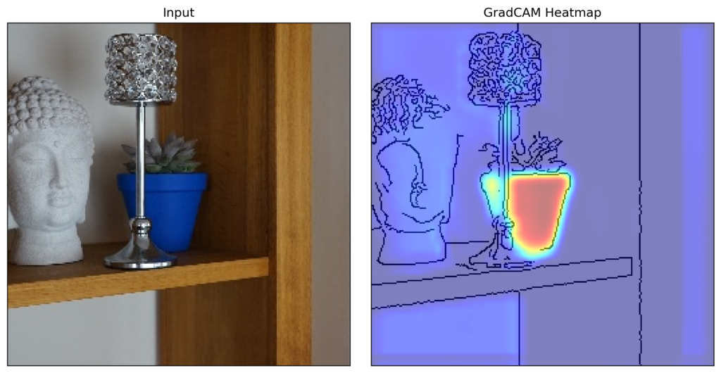
We’ll come back to this conclusion when we discuss the general insights these kinds of heatmaps can bring. For now, let’s see what else we can do with the Grad-CAM package.
Grad-CAM for multiple layers
We can calculate Grad-CAM heatmaps for any of the convolutional layers in the network. On line 2 we have a list of all three of them in our network.
# all conv layers
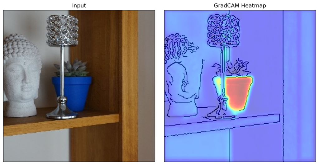
layers = [model.conv_layers[0],model.conv_layers[3],model.conv_layers[6]]We can use the same code as before (lines 2-8). However, keep in mind that this will still produce one heatmap. It will be a weighted average of the heatmaps for the feature maps across all three convolutional layers. You can see the output in Figure 12.
# Get combined heatmap for all layers
cam = GradCAM(model=model, target_layers=layers)
heatmap = cam(input_tensor=image.unsqueeze(0), targets=classes)

# Plot the heatmap
edge = get_canny_edge(rgb_image)
visulaization = show_cam_on_image(edge, heatmap[0], use_rgb=True)
plot_gradcam(rgb_image, visulaization)
Notice that the heatmap is similar to the one for the last layer we saw in Figure 11. There are two potential reasons for this:
- The last layer is given a larger weight. In other words, the gradients of the logit w.r.t. the feature maps are largest for conv3.
- All layers have extracted features with similar spatial information.
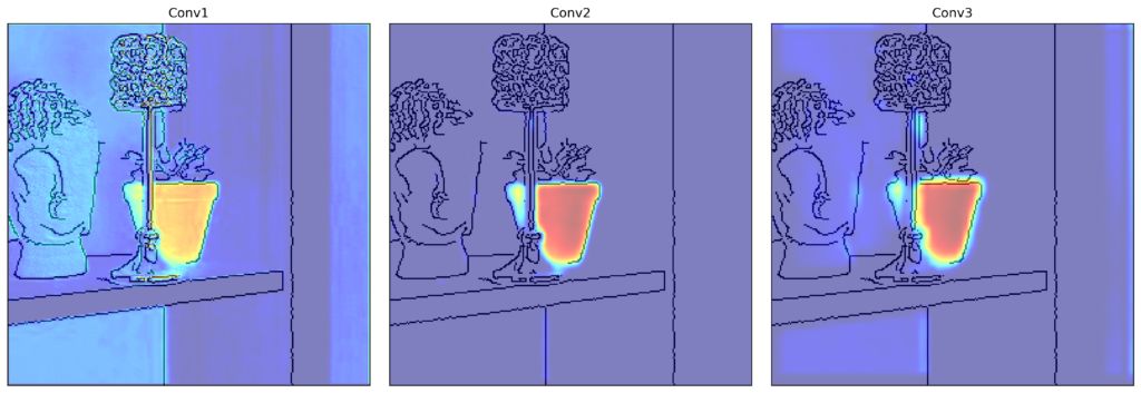
In our case, it is the latter. We can confirm by looping over the list of layers (line 3) and calculating a heatmap for each layer separately (lines 4-6). In Figure 13, we can see the pot is highlighted in all three heatmaps.
# Get seperate visualizations for each layer
maps = []
for layer in layers:
    cam = GradCAM(model=model, target_layers=[layer])
    heatmap = cam(input_tensor=image.unsqueeze(0), targets=classes)
    visulaization = show_cam_on_image(edge, heatmap[0], use_rgb=True)
    maps.append(visulaization)

fig, ax = plt.subplots(1,3,figsize=(15,5))

for i,vis in enumerate(maps):
    ax[i].imshow(vis)
    ax[i].set_title(f"Conv{i+1}")
    ax[i].set_xticks([])
    ax[i].set_yticks([])
When interpreting this plot, we must keep in mind that the insights of Grad-CAM are fundamentally limited. It can only tell us that the locations of the features extracted at the different layers are similar. This does not mean that the same features have been extracted. Typically, earlier layers detect basic patterns and deeper layers detect more abstract features. To see this, we need to use a method like guided backpropagation.
Grad-CAM for multiple classes
It is also possible to calculate heatmaps for multiple classes. On lines 2-5, we have a list of all possible classes for our problem. If we pass this entire list into the cam object it will return one heatmap (line 9). This one will be weighted by the logits/probabilities of the classes.
# Define target classes
classes = [ClassifierOutputTarget(0),
           ClassifierOutputTarget(1),
           ClassifierOutputTarget(2),
           ClassifierOutputTarget(3)]

# Get the GradCAM heatmap
cam = GradCAM(model=model, target_layers=layers)
heatmap = cam(input_tensor=image.unsqueeze(0), targets=classes)
For this instance, the above heatmap will be very similar to what we’ve seen before. This is because the logit for Baya(1) is large relative to the other classes. We can see this when we print the logits for this instance (line 2). This gives us [-2.9944, 9.6644, -0.2042, -2.6261].
# Output scores
print(output)
For our problem, producing combined or separate heatmaps for each of the classes is not useful. However, it can provide useful insight when logits of two classes are close or if the model has made an incorrect prediction. You will be able to see what regions in the image are causing the model to make these mistakes.
Other instances
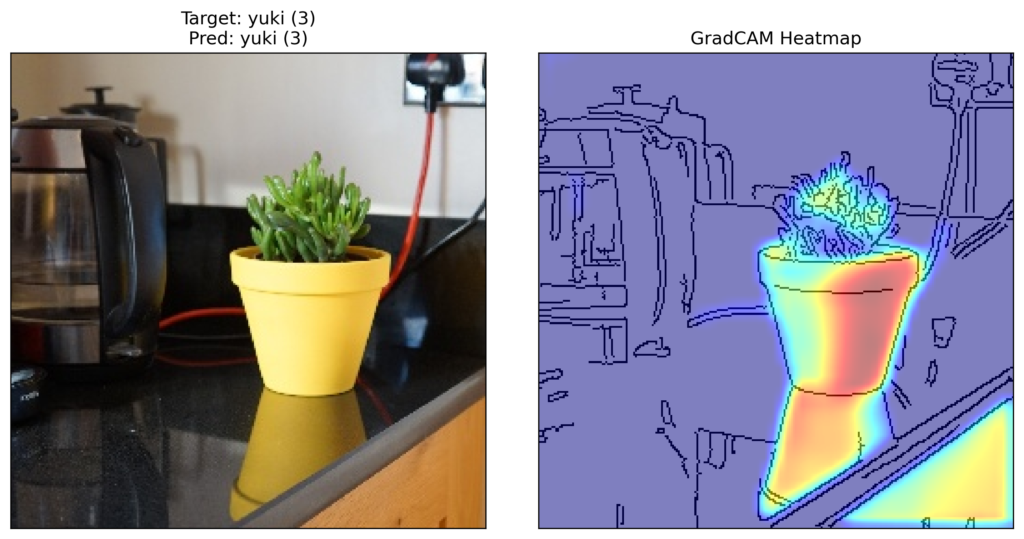
To end, we create heatmaps for a random instance from each of our 4 classes (line 1). For each instance, we use the predicted class (line 20) and the final convolutional layer (line 21). You can see heatmaps for the 4 instances below.
for p in [0,1,2,3]:

    # Get the paths for given class
    paths = glob.glob(base_path + "/test/{}_*.jpg".format(p))

    # Get random instance
    np.random.shuffle(paths)
    data = ImageDataset(paths,num_classes=num_classes)
    image, target = data.__getitem__(0)

    # Format target
    target = torch.argmax(target).item()

    # Get prediction
    input = image.unsqueeze(0).to(device)
    output = model(input)
    pred = torch.argmax(output).item()

    # Use prediction as target class
    classes = [ClassifierOutputTarget(pred)]
    layers = [model.conv_layers[6]]

    # Get heatmap
    cam = GradCAM(model=model, target_layers=layers)
    heatmap = cam(input_tensor=image.unsqueeze(0), targets= classes)

    # Display
    rgb_image = image.permute(1,2,0).numpy()
    edge = get_canny_edge(rgb_image)
    visulaization = show_cam_on_image(edge, heatmap[0], use_rgb=True)

    title = f"Target: {plant_names[target]} ({target})\nPred: {plant_names[pred]} ({pred})"
    plot_gradcam(rgb_image, visulaization,title)
The heatmaps for Rudo(0) and Baya(1) in Figures 14 and 15 are similar to before. The heatmaps for the other two plants in Figures 16 and 17 are slightly more interesting. For Greg(2) and Yuki(3), we can see the model is using some of the actual plants to make predictions.
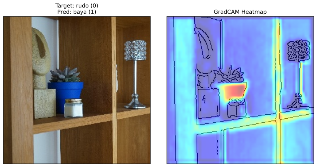
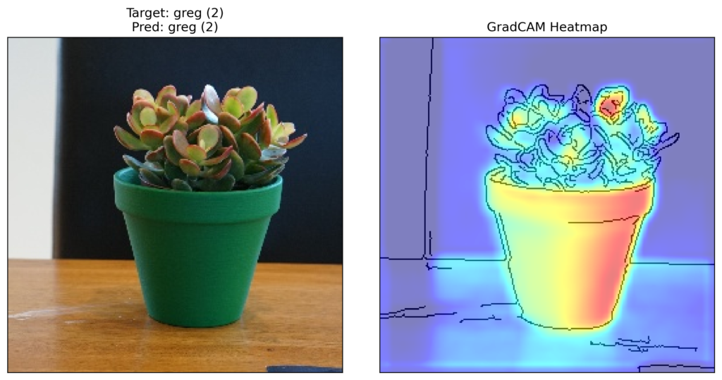
Looking at the above heatmaps we can see that the pots are still significant features for all the instances. As discussed, this is a result of bias introduced into our dataset. The key point is that, if we had not broken Rudo’s pot, we would not have picked up this mistake with evaluation metrics. The same bias would have been present in the training, validation and testing dataset.
Identifying this kind of bias is one benefit of using a method like Grad-CAM. We also discussed some other insights like:
- Understanding the locations of features extracted by different layers in the network.
- Identifying regions in an image causing incorrect predictions for an instance.
All of these insights are valuable as they allow us to develop more robust and efficient models. Ultimately, Grad-CAM can help us correct or improve models before they are put into production.
I hope you enjoyed this article! See the course page for more XAI courses. You can also find me on Bluesky | Threads | YouTube | Medium
Additional Resources
Datasets
Conor O’Sullivan (2024). Pot Plant Dataset. (CC BY 4.0) https://www.kaggle.com/datasets/conorsully1/pot-plants
References
[1] Julius Adebayo, Justin Gilmer, Michael Muelly, Ian Goodfellow, Moritz Hardt, and Been Kim. Sanity checks for saliency maps. Advances in neural information processing systems, 31, 2018.
[2] Harish Guruprasad Ramaswamy et al. Ablation-cam: Visual explanations for deep convolutional network via gradient-free localization. In proceedings of the IEEE/CVF winter conference on applications of computer vision, pages 983–991, 2020.
[3] Ramprasaath R Selvaraju, Michael Cogswell, Abhishek Das, Ramakrishna Vedantam, Devi Parikh, and Dhruv Batra. Grad-cam: Visual explanations from deep networks via gradient-based localization. In Proceedings of the IEEE international conference on computer vision, pages 618–626, 2017.
[4] Kira Vinogradova, Alexandr Dibrov, and Gene Myers. Towards interpretable semantic segmentation via gradientweighted class activation mapping (student abstract). In Proceedings of the AAAI conference on artificial intelligence, volume 34, pages 13943–13944, 2020.
[5] Bolei Zhou, Aditya Khosla, Agata Lapedriza, Aude Oliva, and Antonio Torralba. Learning deep features for discriminative localization. In Proceedings of the IEEE conference on computer vision and pattern recognition, pages 2921–2929, 2016.
Get the paid version of the course. This will give you access to the course eBook, certificate and all the videos ad free.