When you first dive into the swamp of Explainable AI (XAI), the sheer number of methods can be overwhelming. To help bring clarity to the murky pool, we give a structured taxonomy of XAI methods tailored for computer vision. We’re going to discuss the breakdown you see in Figure 1. You may notice that this same breakdown helps define the structure of this course.
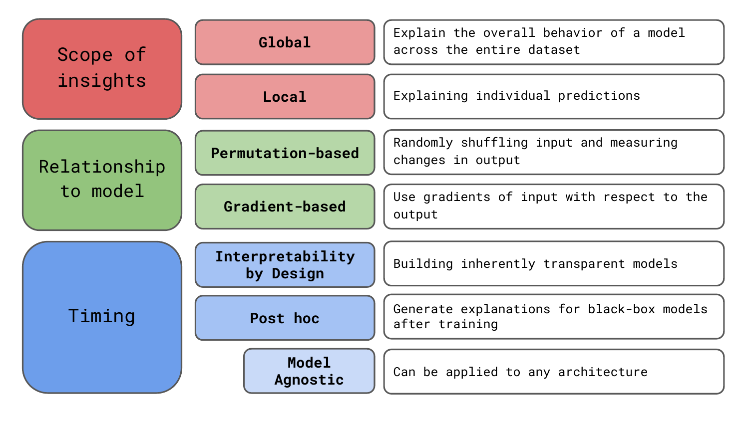
We consider these categories to be the core methodological differences between methods. They help us define the type of insights they offer, their relationship to the underlying model and the timing of their application. However, we should keep in mind that there are other ways of grouping the methods. To end, we discuss some of these, like the granularity of output, sensitivity-based vs contribution-based and axiomatic foundations.
Before you get stuck into the article, here is the video version of the lesson.
Global vs local explainable AI methods
The first way we can classify XAI methods is by the type of insights they offer. Global interpretations aim to explain overall model behaviour. We want to make general claims about model predictions on different segments of instances or the entire dataset. In comparison, local interpretations aim to explain the predictions for individual instances.
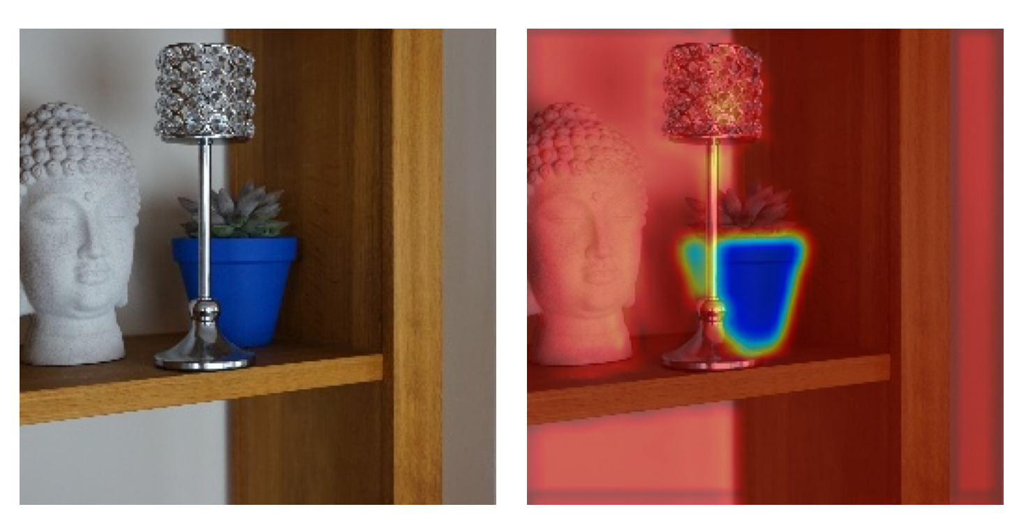
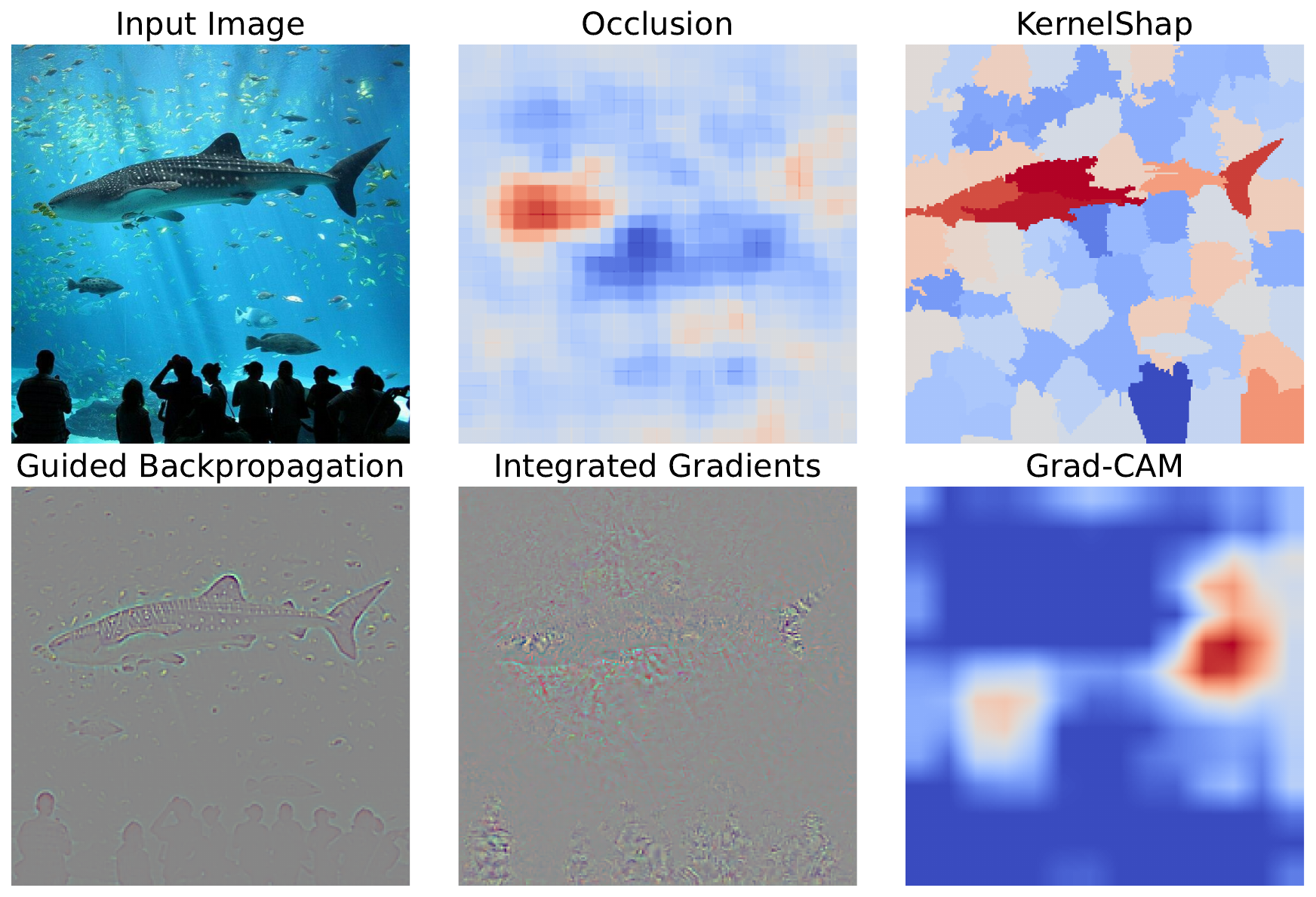
In the context of computer vision, most XAI methods will produce local interpretations. They output a saliency map which shows the pixels in the input image that have contributed the most to the prediction. This is why this book largely revolves around the different mechanisms and properties of various saliency maps. Some of which you can see in Figure 2. These are also commonly referred to as attributions. They attribute a prediction to the features (i.e. pixels) of an image.
To obtain global interpretations, a typical approach is to aggregate saliency maps. For example, we have Grad-CAM heatmaps from a model used to classify X-rays of brain tumours. We could sum the values in different hemispheres or lobes of the brain. Doing this over multiple input images, we can understand which region is more important in general or if the model is biased towards a certain region. Other methods, like weighted context, aggregate the saliency maps of individual pixels in image segmentation models [1]. This is used to quantify how much context is used to classify individual pixels.
Permutation-based vs gradient-based explainable AI methods
The next way we can group XAI methods is by their relationship to the underlying model. Or, in other words, by how they are calculated. The two broad categories are using permutations or looking at the model's gradients.
Permutation-based methods work by systematically or randomly altering pixels in the input and measuring changes in the output. The exact way we do permutations can differ. With permutation channel importance, we will shuffle all pixels in a single channel. With occlusion, we will create saliency maps by systematically replacing regions of an image with neutral values. With SHAP, we will follow a similar process, but by permuting various combinations of regions called superpixels.
Gradient-based methods use the model's gradients acquired by backpropagation. Gradients can be any derivative (or rate of change) of one value w.r.t. another. For most saliency maps, we use the gradients of an output logit w.r.t. the pixels in the input image \(( \frac{\partial y_c}{\partial X} )\). Typically, large absolute gradients indicate that a particular pixel is important to the output. However, as we will see when exploring vanilla gradients, this can produce noisy visualisations.
The remaining methods in the gradient-based section reduce this noise through different mechanisms. For example, Grad-CAM weights the activations in feature maps of a convolutional layer by the average gradients of the map w.r.t. the output. Guided Backpropagation uses ReLU masking to suppress negative gradients, and Integrated Gradients takes an average of gradients computed along a straight-line path from a baseline input to the actual input.
In general, the main benefit of gradient-based methods is that they are significantly less computationally expensive than permutation-based methods. With methods like occlusion, we do multiple (potentially thousands) of forward passes to create saliency maps. For many gradient-based methods, we do only one. On the other hand, permutation-based methods can provide more accurate and less noisy interpretations. As we will discuss in the next section, they can also be used with a larger variety of networks.
Interpretability by design vs post-hoc explainable AI methods
The last way we can group methods is by the timing they are applied. Post-hoc methods are applied after a model is trained. In comparison, interpretability-by-design (IBD) approaches integrate interpretability mechanisms directly into the model’s architecture or decision-making process. In other words, these methods are applied during training.
An example of an IBD method is prototype layers [2]. These work by comparing input features to a learned set of prototypical representations—small, interpretable image patches. The model makes predictions based on the similarity between the input and these prototypes. This makes them easier to understand, as any predictions can be traced back to these human-understandable prototypes.
The downside of IBD methods is that we need to alter the model's architecture. For prototype layers, we need to add new dedicated layers after the convolutional layers. You also need a custom loss function that encourages prototype activation and the separation of prototype layers of different classes. Ultimately, this means that IBD methods are far less flexible and less readily adopted. In comparison, post-hoc methods can be applied to many types of well-established architectures. We explore this trade-off in more detail when comparing Class Activation Maps (CAMs) to Grad-CAM.
Model agnostic methods
We can further distinguish post-hoc methods by whether they are model agnostic. These are methods that can be applied to any architecture as they do not require that we look into their inner workings. So, provided the input and output are the same, we could apply the same method to a feed-forward neural network, CNN or even a transformer.
Permutation-based methods are typically model agnostic. We permute the input image and observe changes in the model's output. At no point do we look at what is happening in the model—it is treated as a black box. Although highly flexible, most gradient-based post hoc methods are not model agnostic. In computer vision, they are typically designed for CNNs only.
Really, when deciding between IBD and post-hoc methods, you should consider your goal. If you want to debug a model before putting it into production, then post-hoc methods are the way to go. They will provide more flexibility when it comes to the architecture, ultimately allowing you to select the one with the best performance.
If you are using deep learning for data exploration, then you can consider IBD methods. In this case, your goal is to learn something new about your dataset or problem and IBD can often provide a unique insight. The lower performance is not necessarily a problem, as you just need a model that captures underlying relationships in the data.
Additional considerations
That covers the main differences in XAI methods. To end, we'll discuss a few other considerations when choosing a method.
Granularity of the output
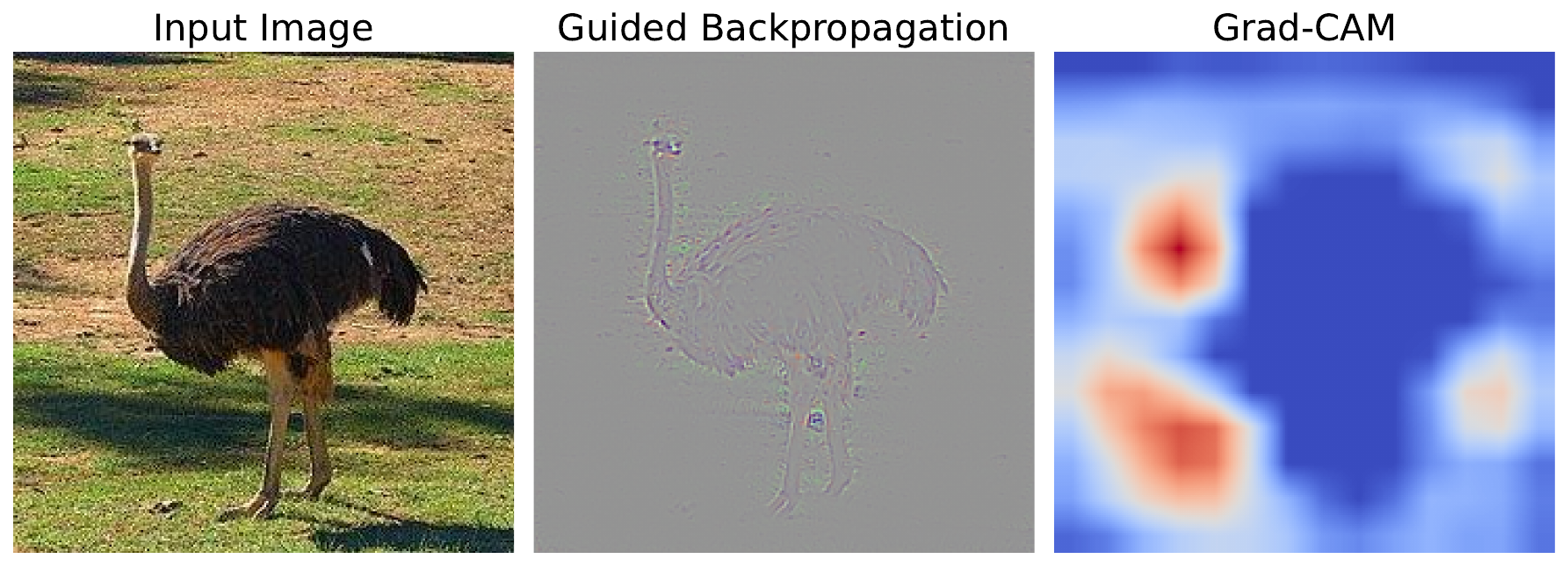
By granularity, we mean how detailed a saliency map is. In Figure 3, you can see that methods like Guided Backpropagation can show detailed features. In comparison, Grad-CAM can only highlight important regions in an image. This is why saliency maps like those generated by Grad-CAM are referred to as heatmaps. The granularity ultimately determines the kind of conclusion you can make from a method.
Sensitivity-based vs contribution-based
As with many terms in machine learning and XAI, there are often conflicting definitions. [3] provides the following definitions:
- Local attribution methods (sensitivity-based): describe how the output of the network changes for infinitesimally small perturbations around the original input.
- Global attribution methods (contribution-based): describe the marginal effect of a feature on the output with respect to a baseline.
These are given in the context of explanations for individual predictions generated using gradient-based methods. This is not the same as the global/local definitions we gave above. The confusion comes as this definition comes from a mathematical context, and is meant to define a model/function in calculus. So to avoid confusion with the previous definition, we refer to these as sensitivity-based vs contribution-based methods.
We talk a bit more about this definition when applying Input x Gradients and the Integrated Gradients method. To summarise, the researchers argue that looking at gradients or an average of gradients alone provides a local interpretation. This is because we can only understand the sensitivity of a function around a given input. When we multiply by the input (\(X\)) or by the difference between the input and baseline (\(X - X^0\)), we obtain a global attribution. This is because we scale the gradients and obtain a cumulative effect.
Axiomatic foundations of explainable AI methods
When we look at the more academic side of XAI, you will encounter different axioms or mathematical properties. We can derive methods from the axioms or prove that a method satisfies the axioms. They include properties like completeness, dummy, symmetry and linearity.
- Completeness: The total attribution across all features should equal the difference between the model output and the baseline prediction.
- Dummy: Features that are missing or do not contribute to a prediction have zero attribution.
- Symmetry: If two features contribute equally to all predictions, they should receive equal attribution.
Axiom-based methods will be derived from a set of axioms or be shown to satisfy a set of axioms. In comparison, heuristic-based methods will produce saliency maps using a simple rule or heuristic. Although the rule usually has a logical justification for why it will produce reasonable saliency maps, the resulting attribution will not necessarily satisfy any axioms. Ultimately, depending on your application, you may need to consider whether a method satisfies these axioms to make more reliable conclusions.
As you can see, there are a lot of considerations when choosing an XAI method. These include the type of insight they offer (global vs local), how they interact with the model (permutation-based vs gradient-based), and when they are applied (post-hoc vs interpretability-by-design). We also discussed model-agnostic methods, the granularity of saliency maps, and the importance of axiomatic foundations.
By understanding these categories, you can better choose the right method for your goals— whether that’s debugging a production model or exploring data-driven insights. As best practice, it’s often useful to apply multiple XAI methods to gain a more robust understanding of your model’s behaviour. Their complementary strengths and weaknesses can often lead to a more complete view of your model.
Challenge
Read about a method called baseline SHAP (BShap) [4]. Classify this method into the three main categories and give the number of axioms it satisfies.
I hope you enjoyed this article! See the course page for more XAI courses. You can also find me on Bluesky | YouTube | Medium
Additional Resources
- Video: What is Explainable AI?
- Video: Model Agnostic Methods
- YouTube Playlist: XAI for Tabular Data
- YouTube Playlist: SHAP with Python
Datasets
Conor O’Sullivan, & Soumyabrata Dev. (2024). The Landsat Irish Coastal Segmentation (LICS) Dataset. (CC BY 4.0) https://doi.org/10.5281/zenodo.13742222
Conor O’Sullivan (2024). Pot Plant Dataset. (CC BY 4.0) https://www.kaggle.com/datasets/conorsully1/pot-plants
Conor O'Sullivan (2024). Road Following Car. (CC BY 4.0). https://www.kaggle.com/datasets/conorsully1/road-following-car
References
- O’Sullivan, Conor, Dev, Soumyabrata (2025). Weighted Context: A Global Interpretation Method for Image Segmentation Models. IGARSS 2025-2025 IEEE International Geoscience and Remote Sensing Symposium, 7082--7086.
- Li, Oscar, Liu, Hao, Chen, Chaofan, et al. (2018). Deep learning for case-based reasoning through prototypes: A neural network that explains its predictions. Proceedings of the AAAI conference on artificial intelligence, 32(1).
- Ancona, Marco, Ceolini, Enea, \"Oztireli, Cengiz, et al. (2017). Towards better understanding of gradient-based attribution methods for deep neural networks. arXiv preprint arXiv:1711.06104.
- Sundararajan, Mukund, Najmi, Amir (2020). The many Shapley values for model explanation. International conference on machine learning, 9269--9278.
Get the paid version of the course. This will give you access to the course eBook, certificate and all the videos ad free.