SmoothGrad
Adding noise to remove noise

The problem: noisy gradients

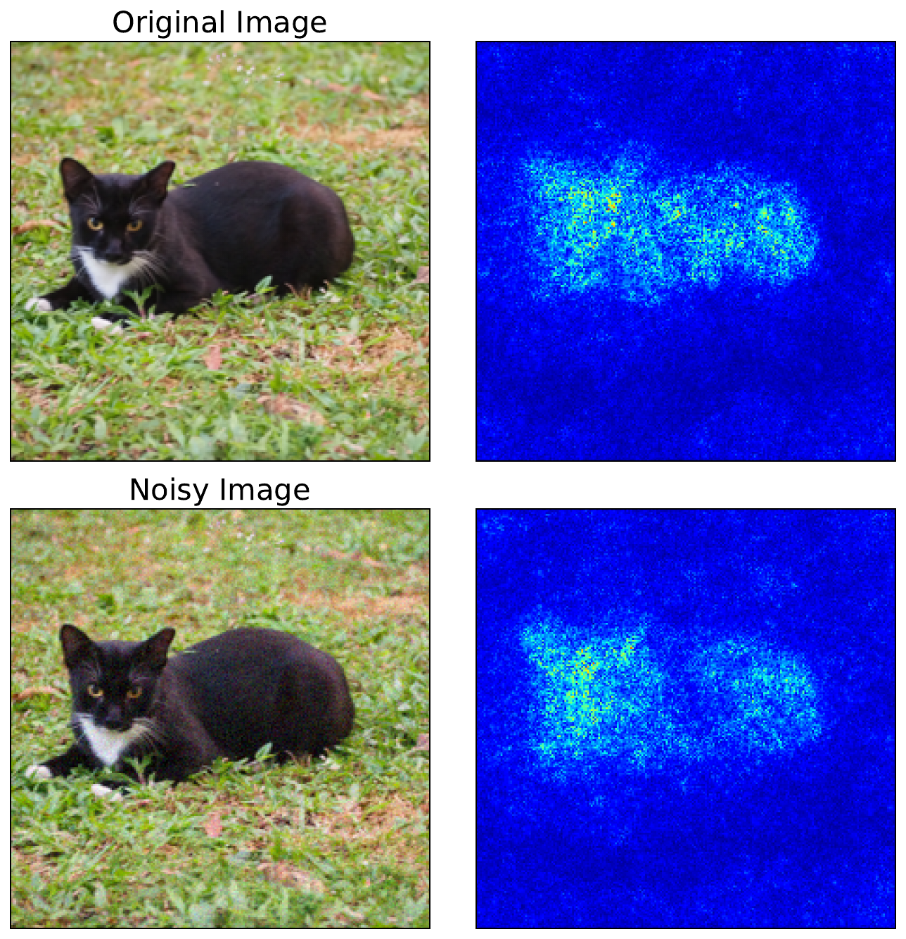
We previously discussed the limitations of Vanilla Gradients. There, we stated that the biggest problem is that gradients can be extremely sensitive to small changes in the input. Small movements in pixel values can lead to large changes in magnitude and even flip the sign of a gradient. You can see this in Figure 1. For the second image, we've added some noise. Although the two images look similar, the resulting saliency maps are different.

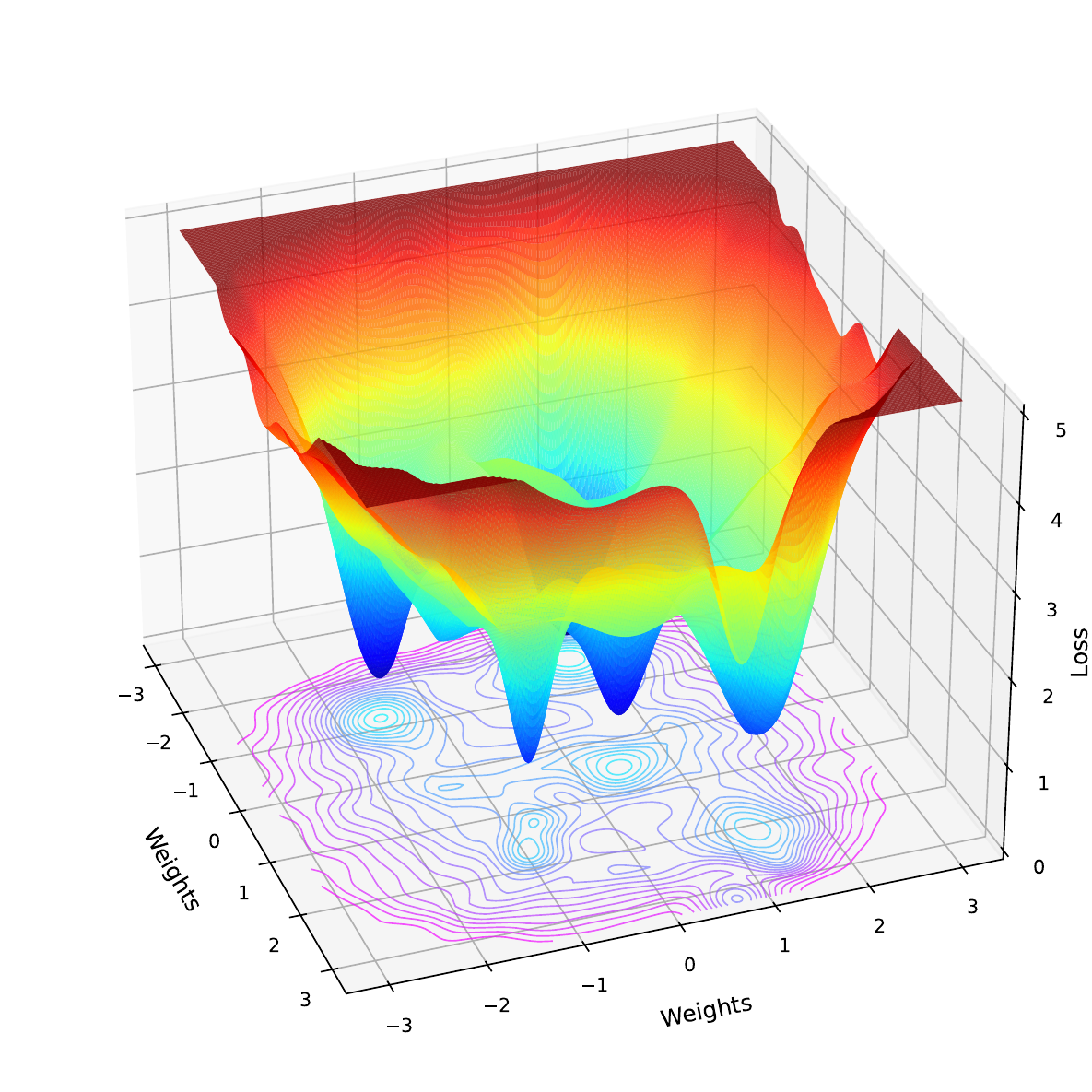
The reason for this is that deep learning models have complex nonlinear decision boundaries. Activation functions like ReLU create sharp boundaries where gradients abruptly switch from zero to non-zero. When a neuron's value crosses one of these thresholds, its gradient can change drastically. Complex interactions between layers can also mean that gradients can behave unpredictably. All this means that the loss functions, like in Figure 2, are rough with many local minima. If we make a small change to the input, we can move to a place on this function where the gradient is significantly different.

The problem is that for any given input, the value for a pixel may be at a position on this jagged landscape that over- or underestimates its importance to the model. This can lead to saliency maps that are hard to interpret, as they will seem random or speckled, even in regions that should be smooth or semantically meaningful. We see this in the saliency maps above, where random background pixels are highlighted.

The solution: adding noise to remove noise

The solution to this problem is summed up in the title of the SmoothGrad paper [1]. We add random Gaussian noise \(\mathrm{N} (0,\sigma^2)\) to our input image (\(X\)) and then calculate the attribution (\(M_c\)) for logit (\(y_c\)) using the augmented input. We do this \(n\) times and take the average. This gives us our final attribution \(\hat{M}_c\).

\[
\hat{M}_c (X) = \frac{1}{n}\sum_n M_c (X + \mathrm{N}(0,\sigma^2))
\]

With each iteration, adding noise to the input causes us to sample gradients from different nearby points on the loss landscape. By averaging these noisy samples, we smooth out the sharp variations in gradients to reveal their general behaviour around the input. When doing this, we have a few choices to make:

• Attribution method (\(M_c\)) - with vanilla gradients (\(M_c(x) = \frac{\partial y_c}{\partial x}\)), but we can use any explanation method.
• Noise level \(\sigma\) - through experimentation the researchers found a standard deviation of between 10% and 20% of an image's pixel range (\(x_{max} - x_{min}\)) produced the best results.
• Iterations \(n\) - similarly, they found that after 50 iterations, the saliency maps converge. To reduce computational time, it may not make sense to go over this amount.

Applying SmoothGrad with Python

To see these choices in action, let's apply SmoothGrad. As mentioned, we'll apply it to Vanilla Gradients as well as Guided Backpropagation (line 9).

import matplotlib.pyplot as plt
import numpy as np

from PIL import Image

import torch
from torchvision import models

from captum.attr import  GuidedBackprop

# Helper functions
import sys
sys.path.append('../')

from utils.visualise import display_imagenet_output, process_attributions
from utils.datasets import preprocess_imagenet_image

Load model and sample image

We'll be using the input image of a goat seen in Figure 3. You can download this image from Wikipedia Commons or using the code in the notebook.

# Load a sample image
img_path = "goat.png"
img = Image.open(img_path).convert("RGB")

plt.imshow(img)
plt.title("Input")
plt.axis('off')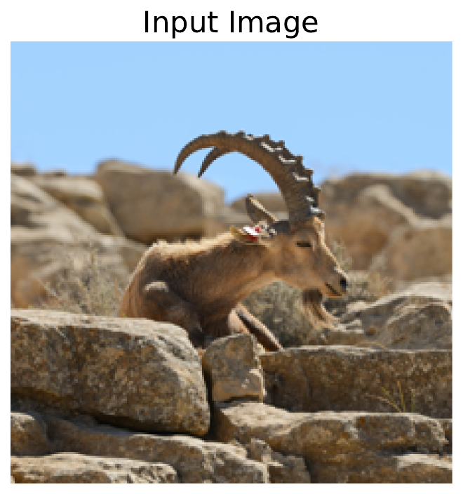

Like in the previous few lessons, we will be using a pretrained model trained on ImageNet. This time we will be using ResNet-50 (line 2).

# Load the pre-trained model (e.g., ResNet50)
model = models.resnet50(pretrained=True)

# Set the model to gpu
device = torch.device('mps' if torch.backends.mps.is_built() 
                      else 'cuda' if torch.cuda.is_available() 
                      else 'cpu')
model.to(device)

# Set the model to evaluation mode
model.eval()
model.zero_grad()

We perform a forward pass using the model and our input image (line 9). In the output, you can see we have close to 100% confidence that this is an image of an ibex (fancy goat). This is the correct prediction, so let's see if we can understand how the model is making it.

# Preprocess the image
original_img_tensor = preprocess_imagenet_image(img_path)
original_img_tensor = original_img_tensor.to(device)

# Clone tensor to avoid in-place operations
img_tensor = original_img_tensor.clone()
img_tensor.requires_grad_() # Enable gradient tracking

predictions = model(img_tensor)

# Decode the output
display_imagenet_output(predictions,n=5)

ibex 0.999991774559021
bighorn 6.572903203050373e-06
ram 7.691302812418144e-07
hare 2.8964134912712325e-07
impala 2.4532033648938523e-07

SmoothGrad + Standard Backpropagation

For comparison, we'll start by getting the gradients using standard backpropagation. This is the exact process we used in the lesson on Vanilla Gradients. That is, we select the logit with the largest value (line 5). We then do a backward pass starting from this logit (line 8).

# Reset gradients
model.zero_grad() 

# We will use this class for all gradient computations
target_class = predictions.argmax()

# Compute gradients w.r.t to logit by performing backward pass
predictions[:, target_class].backward()

This allows us to get the image gradients (line 2). Which we process using our process_attributions function. We'll display the output later after we have obtained it using SmoothGrad.

# Get the gradients
standard_backprop_grads = img_tensor.grad.detach().cpu().numpy()

grads = standard_backprop_grads[0].copy()
grads = process_attributions(grads, activation="abs",skew= 0.5, colormap="viridis")

With SmoothGrad, we are going to repeat the above process 50 times (line 2). Each iteration will use a different randomly augmented image that is created by adding noise to the original image (lines 10 - 12). Specifically, we are adding Gaussian noise with a \(\sigma\) of 15% of the range of the pixel values (line 3). It is not strictly necessary to reset the gradients (lines 15-16), but we do it to be safe.

For each iteration, we will do a backward pass using the augmented image (line 23). Importantly, we always use the same target class from the original image (line 23). This is for the cases when the augmentation may change the prediction. We add the gradients together (line 29) and then find an average (line 31). This is our SmoothGrad attribution.

# Parameters
n_samples = 50  # number of noisy samples
noise_sigma = 0.15 * (img_tensor.max()- img_tensor.min()).item() # standard deviation of noise

# SmoothGrad computation
smooth_grads = torch.zeros_like(original_img_tensor)

for i in range(n_samples):
    # Add noise to original image
    noise = torch.randn_like(original_img_tensor) * noise_sigma 
    noisy_img = original_img_tensor + noise
    noisy_img.requires_grad_()

    # Reset gradients to be safe
    if noisy_img.grad is not None:
        noisy_img.grad.zero_()

    # Forward pass
    preds = model(noisy_img)
    model.zero_grad()

    # Backward pass
    preds[:, target_class].backward()

    # Get gradients
    noisy_grad = noisy_img.grad

    # Accumulate gradients
    smooth_grads += noisy_grad

smooth_grads /= n_samples

# Convert to numpy
smooth_grads_np = smooth_grads.detach().cpu().numpy()[0].copy()

We format the SmoothGrad using the same parameters as the vanilla gradients (line 2). You can see the results from both methods in Figure 4. This is not perfect, but with SmoothGrad, the shape of the animal is clearer, and a lot of the background pixels have become less important. In other words, we have removed the noise.

# Process attribution map (same as your existing function)
smoothgrad_map = process_attributions(smooth_grads_np, activation="abs", skew=0.5, colormap="viridis")

# Visualization
fig, ax = plt.subplots(1, 3, figsize=(12, 6))
ax[0].imshow(img)
ax[0].set_title("Input Image")
ax[1].imshow(grads)
ax[1].set_title("Gradients")
ax[2].imshow(smoothgrad_map)
ax[2].set_title(f"SmoothGrad + Gradients")

for a in ax:
    a.set_xticks([])
    a.set_yticks([])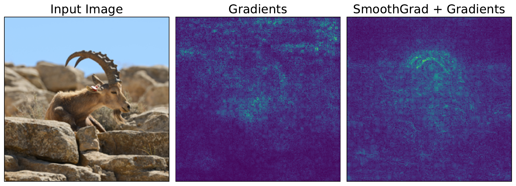

SmoothGrad + Guided Backpropagation

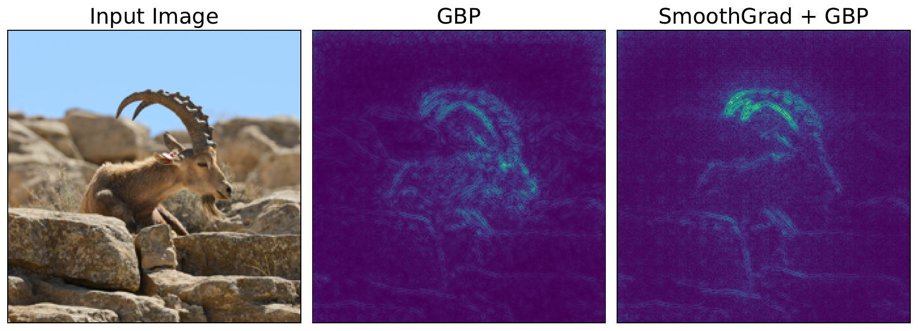
We can apply the exact same process to other attribution methods. Below, we obtain the attribution for Guided Backpropagation (line 6). For each iteration in the SmoothGrad loop, this would replace the code in lines 19 - 26. We can see the output of this in Figure 5.

img_tensor = original_img_tensor.clone()
img_tensor.requires_grad_()

#  Guided Backprop
guided_bp = GuidedBackprop(model)
gb_attr = guided_bp.attribute(img_tensor, target=target_class)

gb_attr = process_attributions(gb_attr, activation="abs", skew=0.5, colormap="viridis")

In this case, SmoothGrad does not impact the visualisation as much. This is because GBP already reduces noise by suppressing negative gradients during the backward propagation. There are still some minor changes, like less background noise. Ultimately, SmoothGrad can still be useful when using more complex gradient-based methods.

The limitations of SmoothGrad

Although SmoothGrad produces cleaner visualisations, we must be aware that it is still a heuristic. This can lead to issues around reliability and faithfulness. Varying the noise level can result in significantly different saliency maps. If we select the one that looks the best, we will be biased towards what a human thinks and not how the model is making a prediction.

SmoothGrad also does not necessarily solve the other big problem of vanilla gradients — saturated gradients. If the pixel is close to a threshold, then minor variations can shift it off that threshold to reveal its importance. However, the variation could be too small to move it out of a flat zone, and the gradients will remain 0 for all variations.

Both of these problems are addressed by the next two methods in this section, DeepLift and Integrated Gradients. Both of these methods are axiom-based attribution methods that use a baseline image. We will see that, for Integrated Gradients especially, this allows the method to satisfy certain desirable properties while leading to a clearer interpretation of the saliency map.

Challenge

Apply SmoothGrad to a different gradient-based method like DeepLIFT or Integrated Gradients.

References

- Smilkov, Daniel, Thorat, Nikhil, Kim, Been, et al. (2017). Smoothgrad: removing noise by adding noise. arXiv preprint arXiv:1706.03825.
Get the paid version of the course. This will give you access to the course eBook, certificate and all the videos ad free.