DeepLIFT
Propogating descrete difference, summation-to-delta rule and Python implementation

With DeepLIFT, we are interested in explaining the difference between the prediction on an input image and a baseline image [1]. The method is essentially a set of rules used to propagate discrete values through a network. We start with the differences in the output logit and work our way back to the input pixels. Along the way, we attribute the differences from the next (deeper) layer to the previous (earlier) layer.

Based on this, it may seem like a mistake to group DeepLIFT with the gradient-based methods. We do this because the process behind the method is similar to backpropagation. Additionally, in practice, the method is applied using a different approach to what was initially presented in the paper [2]. This reformulates DeepLIFT as a modified gradient computation.

To see this, we're going to walk step-by-step through the DeepLIFT rules. We will also demonstrate them using a simple network to better understand how they are used to propagate discrete values. To end the theory section, we discuss some considerations when applying the method, such as how to choose a baseline and which axioms it satisfies. We then move onto applying the method using Captum. Keep in mind, we'll be doing all this for a simple form of DeepLIFT, where positive and negative contributions are combined.

Deltas: what we want to explain

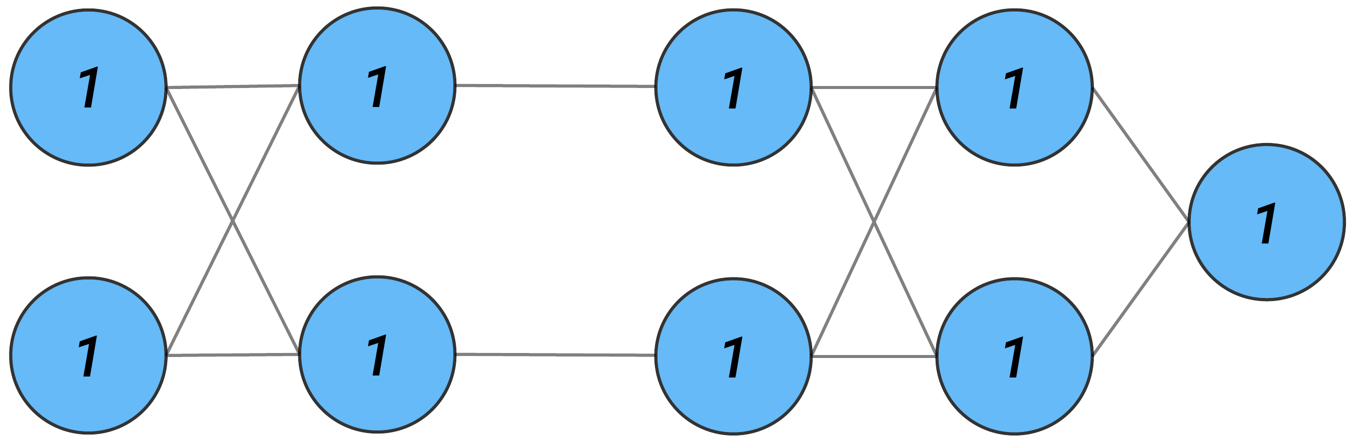
To start, consider the network in Figure 1. We pass the input image through the network to get a value for an output logit, \(y\). This will usually be the logit with the highest value, so let's say this is the logit for the cat class. Like many networks, the value will be a linear sum of the elements in the previous fully connected layer:

\[
y = \sum_i w_i x_i + b
\]

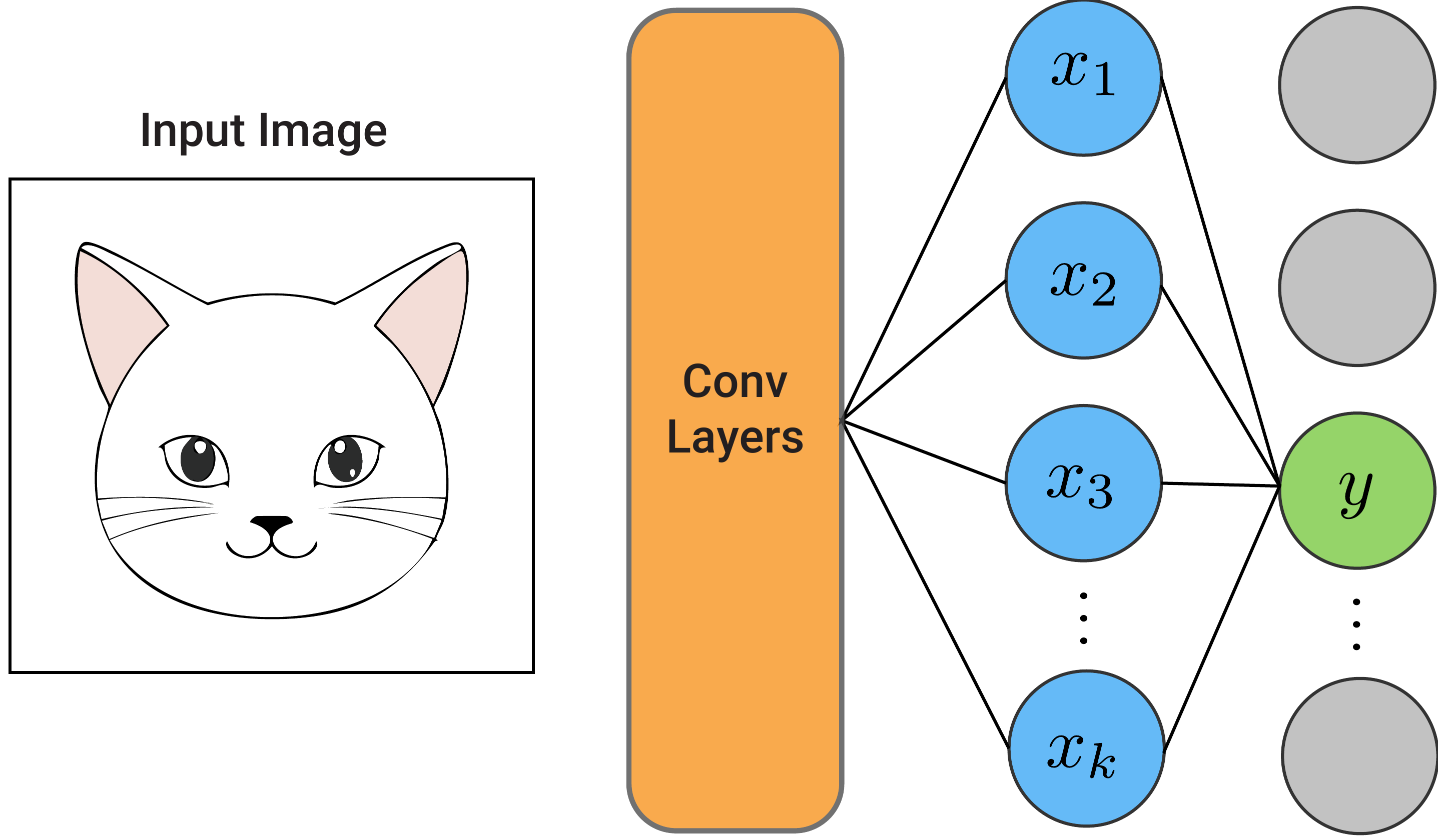
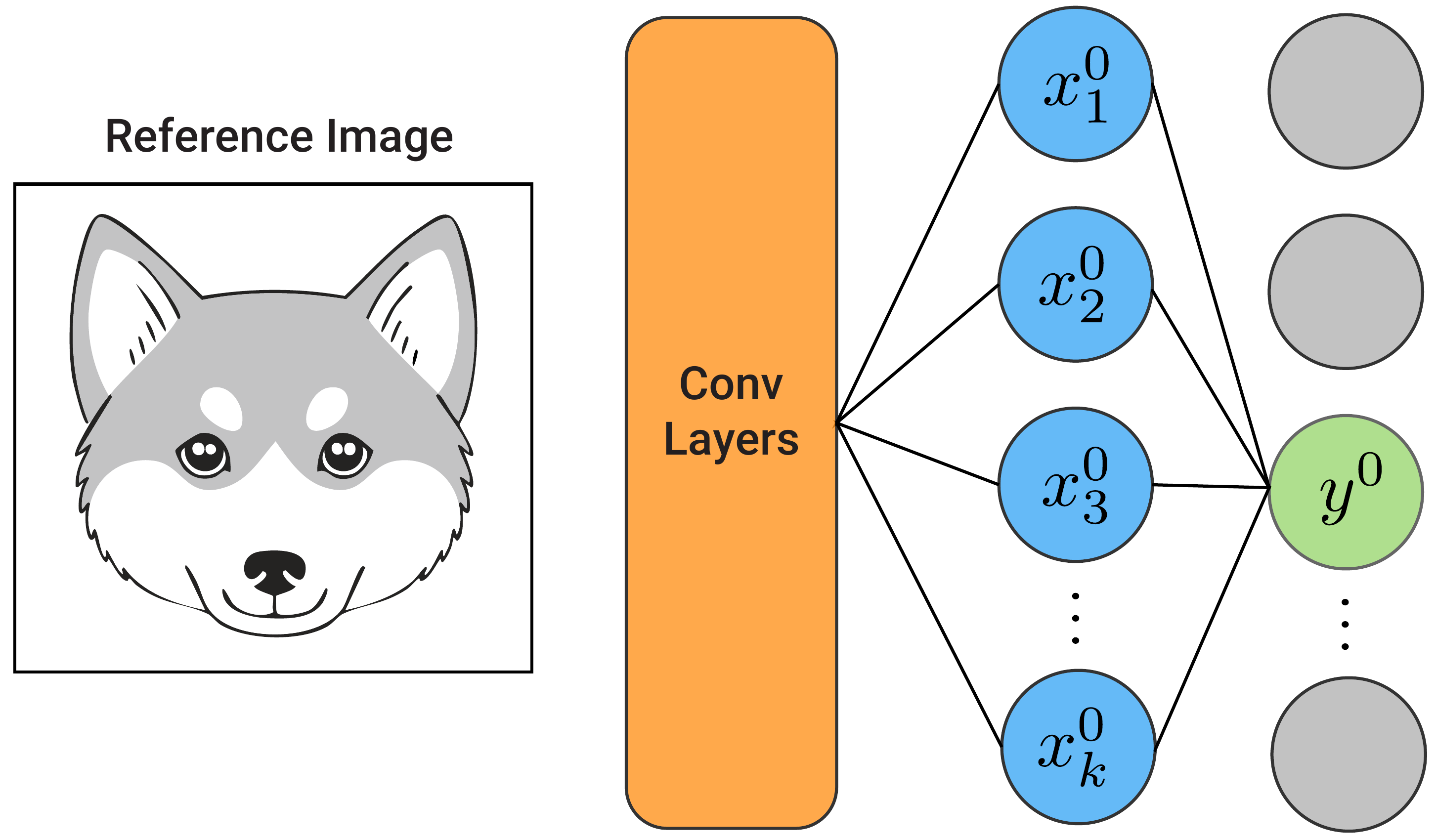
Now, as seen in Figure 2, we pass a baseline image through the same network to obtain \(y^0\). This is the same output logit as before. It will likely have a lower value as we are no longer using a picture of a cat. All the activated elements will also have different values.

Let's focus on the fully connected layer. With DeepLIFT, we want to explain \(\Delta y\). This is the difference in the value of the target logit when we use the input image, \(y\), and the baseline image \(y^0\):

\[
\Delta y = y - y^0
\]

Specifically, we want to attribute \(\Delta y\) to all the \(\Delta x_i\)s. These are the differences in the activated elements of the fully connected layer when we use the input image \(x_i\) and baseline image \(x^0_i\):

\[
\Delta x_i = x_i - x_i^0
\]

We call these values \(C_{\Delta x_i\Delta y}\). They are the contribution of \(\Delta x_i\) to \(\Delta y\). In other words, they tell us how the change in the elements caused the change in the target logit.

\[
C_{\Delta x_i\Delta y} \rightarrow \text{contribution of } \Delta x_i
\]

To find these contributions, DeepLIFT defines rules for calculating and propagating contributions. When doing this, the rules are defined to meet the summation-to-delta property. This is similar to the completeness axiom or efficiency property of SHAP. It requires that all the contributions from a given layer should sum up to \(\Delta y\). In other words, the entire difference in the target logit is explained by the changes in the elements.

\[
\sum_i C_{\Delta x_i\Delta y} = \Delta y
\]

For this fully connected layer, a rule for attributing \(\Delta y\) flows naturally. Consider that:

\[
\begin{aligned}
\Delta y &= y - y^0 \\
&= \sum_k w_i x_i - \sum_k w_i x^0_i \\
&= \sum_k w_i (x_i - x_i^0) \\
&= \sum_k w_i \Delta x_i
\end{aligned}
\]

So, we can maintain the summation-to-delta property if we set:

\[
C_{\Delta x_i\Delta y} = w_i \Delta x_i
\]

This rule is also intuitive. The contribution of each element in the fully connected layer is the change in the element times its weight. Unfortunately, we are usually not that interested in this first layer but in how each of the input pixels has contributed to \(\Delta y\). To do this, we need to define some rules that allow us to propagate discrete contributions back through the network.

DeepLift rules for propagating contributions

When we define the rules, let:

\[
x_i^{(k)} | i = 1,2,3,...,n \rightarrow \text {elements of layer k in the network}
\]

\[
y \rightarrow \text {target logit}
\]

Multipliers

First, we define a multiplier:

\[
m _{\Delta x_i^{(k)}\Delta y} = \frac{C_{\Delta x_i^{(k)}\Delta y}}{\Delta x_i^{(k)}}
\]

This is the ratio of the contribution of the element to the change in the element.

For intermediate layers, they are defined as:

\[
m _{\Delta x_i^{(k)}\Delta x_j^{(k+1)}} = \frac{C_{\Delta x_i^{(k)}\Delta x_j^{(k+1)}}}{\Delta x_i^{(k)}}
\]

In this case, we are considering the contributions of an element in layer \(k\) to those in the next layer \(k+1\).

Chain Rule

You can think of multipliers as the discrete version of gradients, \(\frac{\partial y}{\partial x_i^{(k)}}\). Similar to how gradient descent propagates gradients, we will propagate multipliers. To do this, we define the chain rule:

\[
m _{\Delta x_i^{(k)}\Delta y} = \sum_j m _{\Delta x_i^{(k)}\Delta x_j^{(k+1)}} m _{\Delta x_j^{(k+1)}\Delta y}
\]

Essentially, this means that to calculate the multipliers in the current layer \(k\), we need the multipliers:

• for layer \(k\) to layer \(k+1\)
• for layer \(k+1\) to target logit \(y\)

So, if we define rules for the multiplier from each layer \(k\) to \(k+1\), we can iteratively calculate the multipliers from \(k\) to \(y\). To do that, we use the next two rules.

Linear Rule

Linear layers include fully connected layers and convolutional layers. The value of an element is a linear sum of all its inputs:

\[
x_j^{(k+1)} = b + \sum_i w_i x^{(k)}_i
\]

For these, we define the contributions:

\[
C_{\Delta x_i^{(k)}\Delta x_j^{(k+1)}} = w_i \Delta x_i^{(k)}
\]

The logic behind this is similar to what we discussed with the contributions from the first fully connected layer and the output logit, \(y\). We are saying that the contributions of an element in layer \(k\) are the change in that element multiplied by the weight connecting it to layer \(k+1\).

The multiplier is then:

\[
m_{\Delta x_i^{(k)}\Delta x_j^{(k+1)}} = w_i
\]

These are used to propagate the differences for fully connected layers as well as for convolutional layers. The latter could be thought of as multiple individual linear equations. We need the next rule to handle non-linear layers.

Rescale Rule

A network will consist of various non-linear layers, like ReLU. Specifically, we are considering the layers that take a single value:

\[
x_i^{(k+1)} = f(x_i^{(k)})
\]

As there is only one input, we can attribute the entire change in the element in layer \(k+1\) to the element in layer \(k\). The contributions of all other elements in layer \(k\) will be 0.

\[
C_{\Delta x_i^{(k)} \Delta x_j^{(k+1)}} =
\begin{cases}
\Delta x_j^{(k+1)}, & \text{if } j = i \\[6pt]
0, & \text{if } j \neq i
\end{cases}
\]

The multiplier is therefore:

\[
m_{\Delta x_i^{(k)}\Delta x_i^{(k+1)}} = \frac{\Delta x_i^{(k+1)}}{\Delta x_i^{(k)}}
\]

The DeepLIFT paper proves, mathematically, that if we apply these rules, then the summation-to-delta property is satisfied. That is:

\[
\sum_i C_{\Delta x^{(k)}_i\Delta y} = \Delta y
\]

\[
\sum_i C_{\Delta x^{(k)}_i\Delta x^{(k+1)}_j} = \Delta x^{(k+1)}_j
\]

In other words, we could also use DeepLIFT to understand the contributions to any arbitrary element in the network. We won't go over these proofs, but to show the work rules, we'll apply them to a simple model.

Example using a simple neural network

We're going to apply the DeepLIFT rules to the network in Figure 3. We have our input layer (\(x\)) followed by a fully connected (\(a\)), ReLU (\(b\)), fully connected (\(c\)) and output layer (\(y\)).

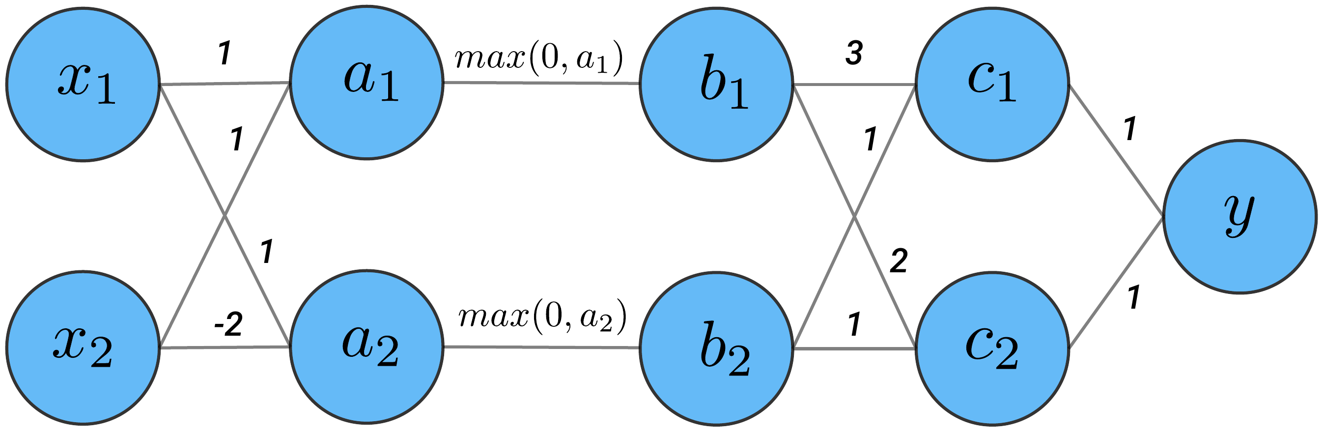
From this network, we have the following linear weights:

\[
\begin{aligned}
w^x_{11} &= 1, & w^x_{12} &= 1 \\
w^x_{21} &= 1, & w^x_{22} &= -2 \\[6pt]
w^b_{11} &= 3, & w^b_{12} &= 2 \\
w^b_{21} &= 1, & w^b_{22} &= 1 \\[6pt]
w^c_{11} &= 1, & w^c_{21} &= 1
\end{aligned}
\]

Figure 4 gives the element values for an input of (1,1). Similarly, Figure 5 gives the values for a baseline of (0,0). We want to understand how the changes in the element values have contributed to the changes in the output.

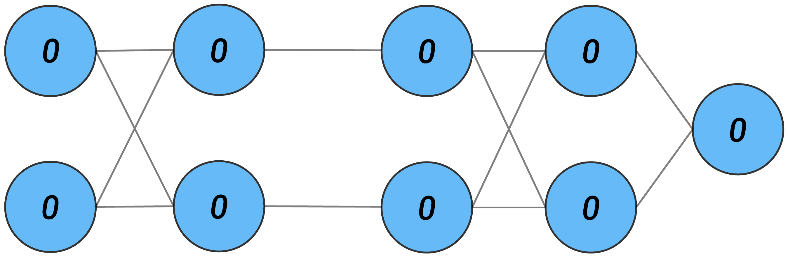
We have the changes (i.e. \(\Delta\)'s) below. As all the values for the baseline elements are 0, these are the same as the values for the instance in Figure 4.

\[
\Delta y = 10 - 0 = 10
\]

\[
\begin{aligned}
\Delta c_1 &= 6, & \Delta c_2 &= 4 \\[4pt]
\Delta b_1 &= 2, & \Delta b_2 &= 0 \\[4pt]
\Delta a_1 &= 2, & \Delta a_2 &= -1 \\[4pt]
\Delta x_1 &= 1, & \Delta x_2 &= 1 \\[4pt]
\end{aligned}
\]

We'll apply the rules defined above to propagate contributions through this network. We will do this until we get the contributions of change in the input features to the change in the output, \(C_{\Delta x_1 \Delta y}\) and \(\quad C_{\Delta x_2 \Delta y}\). As we go, notice that the summation-to-delta property is satisfied for every layer.

Layer \(c\):

\[
\begin{aligned}
m_{\Delta c_1 \Delta y} &= w^c_{11} = 1 && \text{(linear rule)}\\
m_{\Delta c_2 \Delta y} &= w^c_{21} = 1 \\[6pt]
C_{\Delta c_1 \Delta y} &= (\Delta c_1) ( m_{\Delta c_1 \Delta y}) = (6)(1) = 6 \\
C_{\Delta c_2 \Delta y} &= 4 \\[6pt]
\end{aligned}
\]

We have summation to delta:

\[
\sum_j C_{\Delta c_j \Delta y} = 6 + 4 = 10 = \Delta y
\]

Layer \(b\):

\[
\begin{aligned}
m_{\Delta b_1 \Delta y} &= \sum_j m_{\Delta b_1 \Delta c_j} \, m_{\Delta c_j \Delta y}
&& \text{(chain rule)} \\
&= m_{\Delta b_1 \Delta c_1} \, m_{\Delta c_1 \Delta y} + m_{\Delta b_1 \Delta c_2} \, m_{\Delta c_2 \Delta y}\\
&= m_{\Delta b_1 \Delta c_1} \, (1) + m_{\Delta b_1 \Delta c_2} \, (1) && \text{(from above)}\\
&= w^b_{11} + w^b_{12} && \text{(linear rule)}\\
& = 3 + 2 = 5 \\
m_{\Delta b_2 \Delta y} &= w^b_{21} + w^b_{22} = 1 + 1 = 2 \\[6pt]
C_{\Delta b_1 \Delta y} &= \Delta b_1 \, (m_{\Delta b_1 \Delta y}) = 2(5) = 10 \\
C_{\Delta b_2 \Delta y} &= \Delta b_2 \, (m_{\Delta b_2 \Delta y}) = 0(2) = 0
\end{aligned}
\]

Layer \(a\):

\[
\begin{aligned}
m_{\Delta a_1 \Delta y} &= \sum_j m_{\Delta a_1 \Delta b_j} \, m_{\Delta b_j \Delta y} && \text{(chain rule)}\\
&= m_{\Delta a_1 \Delta b_1} \, m_{\Delta b_1 \Delta y} && \text{(one input)}\\
&= m_{\Delta a_1 \Delta b_1} \, (5) && \text{(from above)}\\
&= \frac{\Delta b_1}{\Delta a_1} (5) && \text{(rescale rule)}\\
&= (\frac{2}{2})(5) = 5 \\
m_{\Delta a_2 \Delta y} &= \frac{\Delta b_2}{\Delta a_2} (m_{\Delta b_2 \Delta y}) = (\frac{0}{-1}) (2) = 0 \\[6pt]
C_{\Delta a_1 \Delta y} &= \Delta a_1 ( m_{\Delta a_1 \Delta y}) = 2(5) = 10 \\
C_{\Delta a_2 \Delta y} &= \Delta a_2 ( m_{\Delta a_2 \Delta y}) = (-1)(0) = 0
\end{aligned}
\]

Layer \(x\):

We leave the final fully connected layer as an exercise:

\[
\begin{aligned}
C_{\Delta x_1 \Delta y} & = 5 \\
C_{\Delta x_2 \Delta y} & = 5
\end{aligned}
\]

These tell us that both the change in \(x_1\) and \(x_2\) have contributed 5 units to the change in \(y\). If we go back to the network, these contributions make sense. Both the baseline and input values of \(x_1\) and \(x_2\) are the same. In other words, these values changed by the same amount (\(\Delta x_1 = \Delta x_2\)). Then, for this example, both \(x_1\) and \(x_2\) only influence \(y\) through \(a_1\) where they have the same weight. Ultimately, this shows that we were able to propagate the contribution back to the input in a way that makes sense in the context of this network and instance.

Practical considerations when applying DeepLIFT

Hopefully, you are convinced that the DeepLIFT rules propagate contributions reasonably. We now move on to discussing some important factors you should consider when applying the method. These include different versions of DeepLIFT, situations where summation-to-delta is not satisfied and how the method is actually implemented. To start, we consider an important step when applying the method.

Choosing a baseline

A key feature in DeepLIFT is the use of a baseline image. We are comparing the output from this image to the output from our instance. This helps overcome the issue of saturation and the assumption of local linearity prone to many gradient-based methods. This is because we no longer consider the gradient at a single point, but how the elements change over the distance from the baseline to the input. However, it leaves us with a new problem— how to choose a baseline.

The advice from the DeepLIFT paper is to consider the context of your problem and use domain knowledge. You should ask yourself, "What do I want to compare my prediction to?" Integrated Gradients (IG) also uses a baseline and the advice from that paper is more explicit [3]. They suggest that the baseline should be an instance that produces a near-zero value for the target logit. In other words, the baseline image should provide a complete absence of signal.

In practice, a black, grey or blurred image is often used as a baseline. However, it can often be difficult to achieve a value of 0 for the target logit. It is also important to remember that different baselines can produce different results. This is why it is suggested that you experiment with different baselines. Doing so, we must be aware of the potential bias that can be introduced. It is better to ensure that the resulting explanations agree than to select the one that is visually pleasing or confirms your preexisting beliefs.

Positive and negative contributions

We've been discussing a simplified version of DeepLIFT that was initially presented [4]. We talked about the contributions of \(\Delta x\) to \(\Delta y\), which are propagated using the linear and rescale rules. Later, an additional rule called the reveal-cancel rule was added [1]. This is an alternative rule for propagating contributions of non-linear layers. To implement it, it is necessary to break up contributions into their positive and negative components:

\[
\Delta x = \Delta x^+ + \Delta x^{-}
\]

\[
C_{\Delta x \Delta y} = C_{\Delta x^+ \Delta y} + C_{\Delta x^- \Delta y}
\]

\(\Delta x^+\) is all the positive changes in \(x\). Then, \(C_{\Delta x^+ \Delta y}\) is the contribution of these positive changes to the change in the output. We have a similar interpretation for negative changes. It is suggested that treating these positive and negative terms separately, with the reveal-cancel rule, can produce more intuitive results than the rescale rule. This is demonstrated using specific simplified networks. However, other networks give situations where the rescale rule is preferred.

Ultimately, it is unclear which rule would be better for any given network. This ambiguity is one of the reasons we don't go into detail on this rule or propagating \(\Delta x^+\) and \(\Delta x^{-}\) separately. Another reason is that the Captum implementation we will use also does not currently support this reveal-cancel rule.

DeepLIFT Axioms

DeepLIFT can be thought of as an axiom-based method as it was designed to satisfy the summation-to-delta (i.e. completeness) axiom. Rules are provided for linear and non-linear components of a single variable. However, it has been shown that, for some implementations, the method does not satisfy completeness when the network has multiplicative interactions [2]. These are common in RNNs. In other words, the method is closer to being a heuristic than axiom-based.

In the lesson on IG, we do a more thorough comparison to DeepLIFT. For now, know that IG does satisfy the completeness axiom, and many others, for all networks. So, if you are concerned with axioms, then it is likely a better option. Still, DeepLIFT is a less computationally expensive method, and as we will discuss in the next lesson, it can often provide a good approximation for IG attributions. This is related to how DeepLIFT is implemented.

Captum Implementation

The process we've walked through above involves propagating discrete differences through the network. However, when we go on to apply the method, this is not how the saliency maps are actually calculated. This is because it has been proved that DeepLIFT attributions can be calculated using gradients [2]. That is, by modifying the gradient functions, they can calculate the same attributions using backpropagation as those that are calculated using rules defined in the original DeepLIFT paper.

This significantly simplifies the implementation of the method. For PyTorch, it means we can rely on the computation graph instead of defining individual rules for every type of layer. As the researchers point out, it also provided a unified framework for comparing different gradient-based methods, like DeepLIFT and IG. Which, as just mentioned, provides some insights when comparing the two methods. For now we will move onto using this implementation.

Applying DeepLIFT with Captum

[Python video coming soon]

As always, we start with our imports. We're going to be importing a model and data processing class from Hugging Face (line 7). We will also use the DeepLift attribution method provided by Captum (line 9).

import matplotlib.pyplot as plt
import numpy as np

from PIL import Image,ImageFilter

import torch
from transformers import AutoModelForImageClassification, AutoImageProcessor

from captum.attr import DeepLift

#Helper functions
import sys
sys.path.append('../')

from utils.visualise import process_attributions, get_edge, add_edge_to_attributions

Load model from Hugging Face

We will be working with the resnet18-catdog-classifier.This model is the pretrained ResNet-18 architecture that has been fine-tuned to classify images as either a cat or a dog. We load the model (line 3) and the associated data processing function (line 4). This is used to process images (e.g. normalize, convert to tensor) so they are in the correct format for the model.

# Load model and processor
model_name = "hilmansw/resnet18-catdog-classifier"
base_model = AutoModelForImageClassification.from_pretrained(model_name)
processor = AutoImageProcessor.from_pretrained(model_name)
base_model.eval()

Now, the DeepLIFT attribution method expects the output of a model to be a single tensor of logits. However, our model outputs a dataclass with additional fields. To address this, we wrap the model (lines 2-10) so that only the logits are returned as output (line 8). Finally, we zero the gradients of the model, just in case there are some left over from training or evaluation (line 11).

# Wrap model to return only logits
class WrappedModel(torch.nn.Module):
    def __init__(self, model):
        super().__init__()
        self.model = model
    def forward(self, x):
        outputs = self.model(x)
        return outputs.logits  # Captum needs a Tensor output

model = WrappedModel(base_model)
model.zero_grad()

Load input images

We'll be working with two images – one of a cat and one of a dog. You can see these in Figure 6. You can download these images from Wikimedia Commons and there is code in the notebook that will do it automatically for you.

# Update paths
cat_img = Image.open("cat.png")
dog_img = Image.open("dog.png")

fig, ax = plt.subplots(1, 2, figsize=(8, 4))

ax[0].imshow(cat_img)
ax[0].set_title("Cat", size=20)

ax[1].imshow(dog_img)
ax[1].set_title("Dog", size=20)

for a in ax:
    a.set_xticks([])
    a.set_yticks([])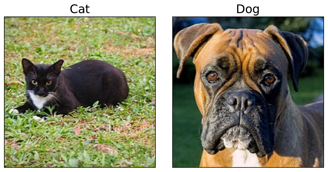

We process these images so they can be used as input into the model (lines 2-3).

# Load and preprocess images
cat_inputs = processor(images=cat_img, return_tensors="pt",crop_pct=1.0)
dog_inputs = processor(images=dog_img, return_tensors="pt",crop_pct=1.0)

print(cat_inputs['pixel_values'].shape)  # Should be [1, 3, 224, 224]
print(dog_inputs['pixel_values'].shape)  # Should be [1, 3, 224, 224]

We do a forward pass with the cat image (lines 2-4). This shows us we have the correct prediction and that the cat class is given by index 0. Now let's explain this prediction using DeepLIFT.

# Forward pass
with torch.no_grad():
    logits = model(cat_inputs["pixel_values"])
    predicted_class_idx = logits.argmax(-1).item()

    print("Logits:", logits)
    print(f"Class idx: {predicted_class_idx}")
    print(f"Class:", base_model.config.id2label[predicted_class_idx])

Logits: tensor([[ 7.3466, -7.1000]])
Class idx: 0
Class: cats

DeepLIFT attributions with various baselines

We're going to apply DeepLIFT with four different baselines – zero, mean, blurred and another input image. We'll use the function below to plot each of these. Let's start with the zero baseline.

def plot_attributions(input_img,baseline,attr):

    fig, ax = plt.subplots(1, 3, figsize=(10, 4))

    # Input
    ax[0].imshow(input_img)
    ax[0].set_title("Input")

    #Baseline
    ax[1].imshow(baseline)
    ax[1].set_title("Baseline")

    # attribution
    ax[2].imshow(attr)
    ax[2].set_title("DeepLift Attribution")

    for a in ax:
        a.set_xticks([])
        a.set_yticks([])

Zero baseline

We start by initializing the DeepLIFT attributions object (line 2). This requires us to pass our model into the DeepLift function.

# Initialize DeepLift
deeplift = DeepLift(model)

We then create our baseline image of all zeros (line 1) and apply the same processing as any input image (line 2). We then pass this (line 7) along with our input tensor (line 6) and target class (line 8).

zero_baseline = np.zeros_like(cat_img)
zero_baseline_tensor = processor(images=zero_baseline, return_tensors="pt",crop_pct=1.0)

# Compute attributions (cat vs zero)
attributions = deeplift.attribute(
    inputs=cat_inputs["pixel_values"],
    baselines=zero_baseline_tensor["pixel_values"],
    target=0
)

We format the attributions using the function. If you missed it, we discussed this function in the lesson on Vanilla Gradients. We also use the get_edge function we discussed in the lesson on Grad-CAM. The final result can be seen in Figure 7. Notice that, in this case, the eyes of the cat seem important to the prediction.

attr = process_attributions(attributions,activation='abs',skew=0.5,colormap='jet')

cat_edge = get_edge(cat_img,h1=0.2,h2=0.3,sigma=5)
attr = add_edge_to_attributions(attr,cat_edge,'white')

baseline = np.zeros((224,224,3))
plot_attributions(cat_img,baseline,attr)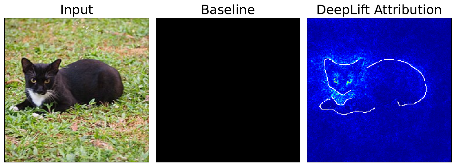

Mean baseline

Before we move on to the mean baseline, we must remember that the processing function applies the standard normalization values for ImageNet. That is:

mean = [0.485, 0.456, 0.406]
std  = [0.229, 0.224, 0.225]

So we can define a mean baseline using the code below. The result is an image where every pixel has the same value as the mean from ImageNet.

# Equivalent to using this tensor
mean_baseline = np.ones_like(cat_img, dtype=np.float32)
for i in range(3):
    mean_baseline[:,:,i] *= [0.485, 0.456, 0.406][i]

However, we would still need to process this image using the same methods as the input image. If we did this using the processor function, the normalization means we would end up with a tensor of zeros (or close to zero after rounding differences). In other words, it is simpler to use a tensor of all zeros straight away.

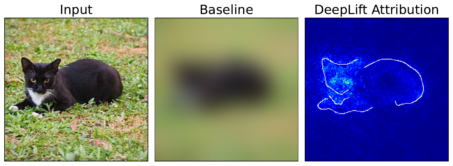
This is actually the default value used by the DeepLIFT attribution object if no baseline is provided (lines 2-5). We process the attribution in the same way and you can see the output in Figure 8. The eyes still seem important, but now the face and parts of the body are also contributing to the difference between the input and the mean baseline.

# Mean baseline
attributions = deeplift.attribute(
    inputs=cat_inputs["pixel_values"],
    target=0
)

attr = process_attributions(attributions,activation='abs',skew=0.5,colormap='jet')
attr = add_edge_to_attributions(attr,cat_edge,'white')
plot_attributions(cat_img,mean_baseline,attr)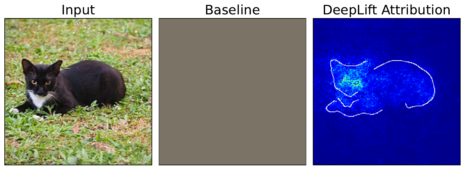

Blurred baseline

Another popular baseline is to use a blurred version of the input image. We obtain this by applying a Gaussian blur (line 1) and processing as before (line 2).

blurred_baseline = cat_img.filter(ImageFilter.GaussianBlur(radius=15))
blurred_baseline_tensor = processor(images=blurred_baseline, return_tensors="pt",crop_pct=1.0)

# Compute attributions (cat vs blurred)
attributions = deeplift.attribute(
    inputs=cat_inputs["pixel_values"],
    baselines=blurred_baseline_tensor["pixel_values"],
    target=0
)

attr = process_attributions(attributions,activation='abs',skew=0.5,colormap='jet')
attr = add_edge_to_attributions(attr,cat_edge,'white')
plot_attributions(cat_img,blurred_baseline,attr)

Looking at the output in Figure 9 you can see that the eyes and face are important. This is potentially because the finer details, like the eyes and whiskers, are removed with blurring. In comparison, the shape and colour of the body are still visible in the blurred image. In other words, these areas do not change as much between the input and baseline.

Another input image as baseline

The final option is to use another input image as a baseline. In this case, we would investigate questions like why one image is classified as a given class and another as a different class. This could be particularly useful if you are trying to understand edge cases, like similar images where one has an incorrect prediction.

For this baseline, we initialize a new DeepLIFT object (line 2). The difference is that we are no longer multiplying the attribution by the difference in the input and baseline. We touch on this in more depth in the section on Integrated Gradients. In this case, we do it as it produces a clearer visualisation.

# Initialize DeepLift
deeplift = DeepLift(model,multiply_by_inputs = False)

We follow the same process as before, using the dog tensor as a baseline (line 4). You can see the output in Figure 10.

# Compute attributions (cat vs dog)
attributions = deeplift.attribute(
    inputs=cat_inputs["pixel_values"],
    baselines=dog_inputs["pixel_values"],
    target=0
)

# Combine dog and cat edge
dog_edge = get_edge(dog_img,h1=0.3,h2=0.4,sigma=2)
edge = np.clip(cat_edge+dog_edge,0,1)

attr = process_attributions(attributions,activation='abs',skew=0.5,colormap='jet')
attr = add_edge_to_attributions(attr,cat_edge,'white')
attr = add_edge_to_attributions(attr,dog_edge,'black')
plot_attributions(cat_img,dog_img,attr)

The interpretation of this output is more complicated than before. It tells us which pixels have contributed to the difference in the predicted logit for the cat class when the input image changes from an image of the cat to a dog. In this case, it looks like the eyes of the dog are important. However, we should keep in mind that it is difficult to distinguish which of the attributions are due to the dog features or the cat features. It is likely a combination of both of them.

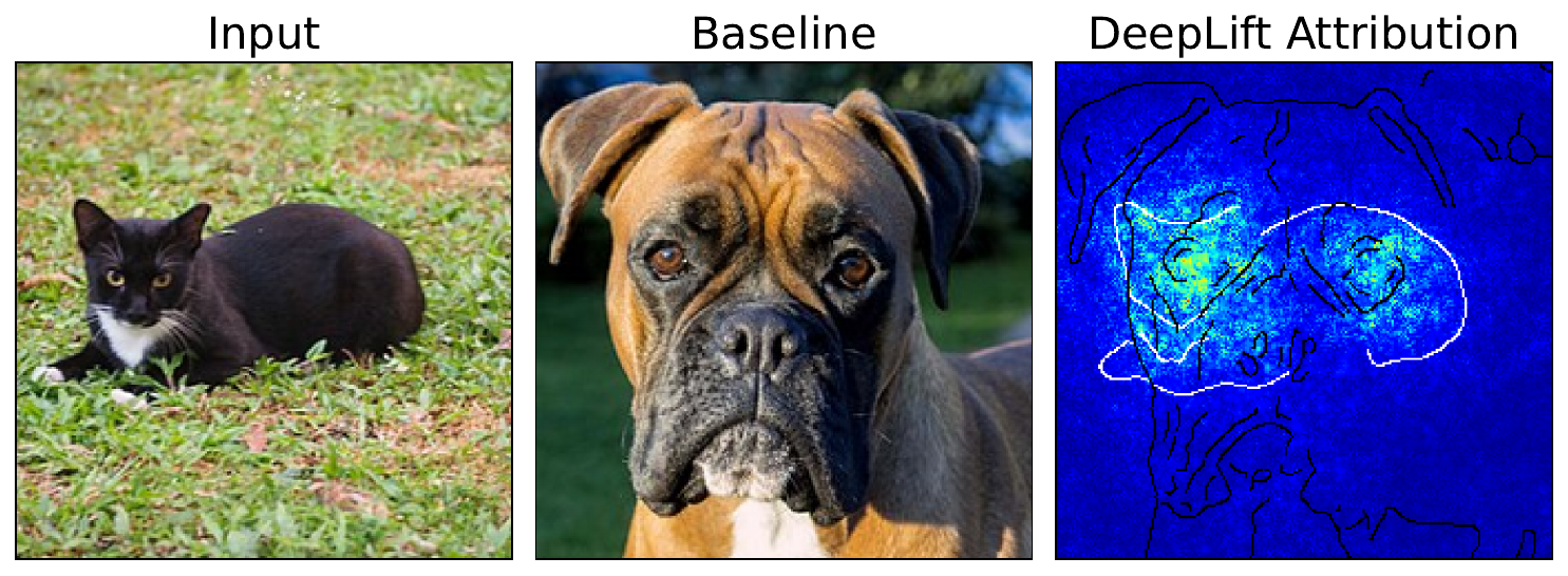
Ultimately, what you should remember is that DeepLIFT can produce different attributions depending on the baseline. This is a known issue with baseline methods in general. It means that you may want to experiment with a few different baselines to be more certain about which features are important to a prediction.

Challenge

Apply the same set of baseline images for using the dog as the input image.

References

- Shrikumar, Avanti, Greenside, Peyton, Kundaje, Anshul (2017). Learning important features through propagating activation differences. International conference on machine learning, 3145--3153.
- Ancona, Marco, Ceolini, Enea, Oztireli, Cengiz, et al. (2017). Towards better understanding of gradient-based attribution methods for deep neural networks. arXiv preprint arXiv:1711.06104.
- Sundararajan, Mukund, Taly, Ankur, Yan, Qiqi (2017). Axiomatic attribution for deep networks. International conference on machine learning, 3319--3328.
- Shrikumar, Avanti, Greenside, Peyton, Shcherbina, Anna, et al. (2016). Not just a black box: Learning important features through propagating activation differences. arXiv preprint arXiv:1605.01713.
Get the paid version of the course. This will give you access to the course eBook, certificate and all the videos ad free.