Convolutional neural networks (CNNs) make decisions using complex feature hierarchies. It is difficult to unveil these using methods like occlusion, SHAP and Grad-CAM as they focus on regions of important pixels. Guided Backpropagation (GBP) addresses this by visualizing the specific features that contribute to a model’s output [1]. It does this by modifying the standard backpropagation process to pass only positive gradients that contribute to a prediction.
We explore three ways to compute and interpret GBP gradients. These are the gradients of a:
- Target logit w.r.t. the input \( \left( \frac{\partial y_c}{\partial X} \right) \) – this helps identify which parts of an image contribute most to a class prediction.
- Target logit w.r.t. the intermediate feature maps \( \left( \frac{\partial y_c}{\partial A} \right) \) – this helps us understand the role of different layers in the network.
- Element in a feature map w.r.t. the input \( \left( \frac{\partial A_{ij}}{\partial X} \right) \) – this reveals the spatial properties of abstract features learned by deeper network layers.
Each of these approaches offers unique benefits to interpreting a model. As we go, they will also provide an intuitive understanding of how CNNs work and how methods like Grad-CAM can use the spatial nature of feature maps.
To implement these methods, we will use PyTorch hooks. As you will see, these allow us to extract gradients and activations dynamically during forward and backward passes. By the end, you will have a practical understanding of guided backpropagation and how to interpret its gradients.
Interested in XAI? Check out one of these courses to learn more:
A note on terminology
Before we start, let’s clarify a few terms:
- Activations are the output from any layer in the network during a forward pass. For example, the raw values from convolutional layers or the after those values have been passed into an activation function.
- Similarly, a feature map is one channel in the output of a convolutional layer or after that layer has been passed to an activation function.
- An element is one unit/pixel in a feature map.
We can talk about activated feature maps if they have been activated by a forward pass. However, we can also refer to them simply as feature maps. Whether they are activated or not should be clear by the context.
The theory behind guided backpropagation
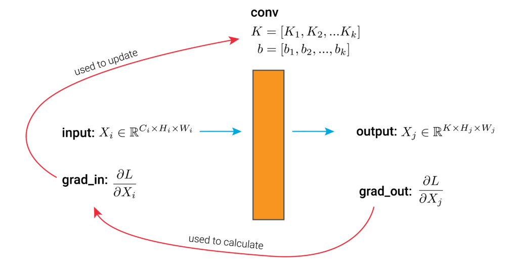
To understand Guided Backpropagation, we start with the standard backpropagation procedure for a convolutional layer seen in Figure 1. This consists of a set of kernels, \(K\), and biases, \(b\). The other parts are the:
- input – set of feature maps or image
- output – set of feature maps
- grad_in is the gradient of the loss w.r.t. the layer’s input.
- grad_out is the gradient of the loss w.r.t. the layer’s output.
We have labelled these using the same variable names as the hook functions that we apply later. This should help connect the theory to the practical application.
During the forward pass, the layer will apply the kernels and biases to the input to produce a new set of feature maps as output. Without going into detail, during the backward pass, grad_out is passed from the next layer in the network. We use this to help calculate grad_in. grad_in is then used to help update the current layer’s kernels and biases.
For GBP, we are not concerned with the final step (i.e. updating the parameters). We only want to visualise the gradients flowing through the network for one input image. When doing this, we make one adjustment to standard backpropagation. That is to only allow positive gradients to flow through ReLU activation layers. A process called ReLU masking.
ReLU masking in guided backpropogation
To understand ReLU masking, we need to introduce the concept of a guidance signal. This is anything that helps reduce noise in a saliency map or guides the visualization toward features that positively contribute to the model’s prediction.
With standard backpropagation, ReLU layers already introduce one guidance signal. That is if the activation from the forward pass is negative the gradient from the backwards pass is set to zero. ReLU masking adds an additional guidance signal. That is, if the gradient flowing backward is negative, it is set to zero.
Looking at Figure 2, you can see the process for standard backpropagation for a ReLU activation layer. During the forward pass, the input is feature maps from the previous convolutional layer. The output will be those same feature maps but with all negative values set to zero.
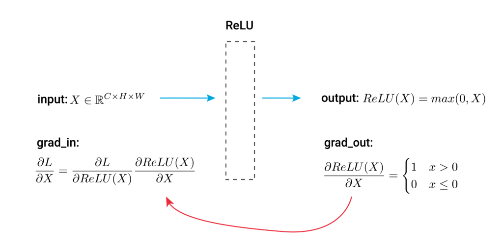
Using the chain rule, we can express grad_in as:
\[\frac{\partial L}{\partial X} = \frac{\partial L}{\partial \text{ReLU}(X) } \cdot \frac{\partial \text{ReLU}(X) }{\partial X} \]
The derivative of the ReLU function can be simplified to:
\[\frac{\partial \text{ReLU}(X) }{\partial X} =
\begin{cases}
1, & X > 0 \\
0, & X \leq 0
\end{cases} = \mathbf{1}(X > 0) \]
This is the guidance signal from standard backpropagation. We only pass gradients through ReLU activation functions where the input is positive. Keep in mind that this does not mean we only pass positive gradients. This is because \( \frac{\partial L}{\partial \text{ReLU}(X) }\) can be both positive and negative regardless of whether the elements of the input feature maps are positive or negative.
\[ \frac{\partial L}{\partial X} =
\frac{\partial L}{\partial \text{ReLU}(X) } \cdot \mathbf{1}(X > 0) \]
So, with guided backpropagation, we introduce an additional guidance signal, \(\mathbf{1}\left( \frac{\partial L}{\partial \text{ReLU}(X) } > 0 \right)\). This will set all negative gradients to 0. These modified gradients are then propagated through the network.
\[ \frac{\partial L}{\partial X} = \frac{\partial L}{\partial \text{ReLU}(X) } \cdot \mathbf{1}\left( \frac{\partial L}{\partial \text{ReLU}(X) } > 0 \right) \cdot \mathbf{1}(X > 0) \]
When we do Guided Backpropagation, we are typically not interested in \(\frac{\partial L}{\partial X}\) but \(\frac{\partial y_c}{\partial X}\). That is the gradients of an output logit for a given class \(c\)(usually, the class with the highest logit). To start the backward pass from this logit, we set \( \frac{\partial L}{\partial y_c} = 1 \) and all \( \frac{\partial L}{\partial y_j} = 0 \). The ReLU masking process is the same as before.
\[\frac{\partial L}{\partial X} = \frac{\partial L}{\partial y_c}\frac{\partial y_c}{\partial X} + \sum_{j \neq c } \frac{\partial L}{\partial y_j}\frac{\partial y_j}{\partial X} = \frac{\partial y_c}{\partial X}\]
To summarise, Guided Backpropagation works by modifying the ReLU activation functions in a CNN so that all negative gradients are set to 0. These layers will now suppress gradients passed during back propagation in two ways, those where the:
- input is negative (standard backprop)
- gradient is negative (guided backprop)
Now, let’s try to understand why this trick works so well.
The intuition behind guided backpropagation
There is no mathematical or fundamental theorem for why Guided Backpropagation should produce better visualisations. In the paper that presented the method, the researchers compare the approach to standard backpropagation and deconvolution — two alternative approaches for creating similar saliency maps. They observed that GBP produced “cleaner visualisations” [1]. The intuition for this can also be found in the paper:
We call this method guided backpropagation, because it adds an additional guidance signal from the higher layers to usual backpropagation. This prevents backward flow of negative gradients, corresponding to the neurons which decrease the activation of the higher layer unit we aim to visualize.
As discussed, standard backpropagation already has one guidance signal. That is, only gradients where the activated feature map has positive elements are propagated. This reduces the number of irrelevant gradients as we only pass those for elements that have increased the predicted logit of the target class.
However, we will still pass negative gradients. In standard backpropagation, negative gradients play a crucial role in reducing the activation of elements that are not associated with the target class. When it comes to GBP, we are only interested in visualising elements that are associated with the target class. So, by suppressing negative gradients, we can reduce noise and create cleaner visualisations.
Intuitively, this makes sense. However, the lack of a theoretical foundation is one of the weaknesses GBP. It means the method is more likely to lead to saliency maps that are incorrect or misleading. This is something we discuss in more depth in the lesson on integrated gradients. Keep that in mind when you apply the method.
Applying guided backpropagation with PyTorch hooks
We start with our imports. We don’t have a package for Guided Backpropagation as we will be applying the method from scratch. If you do want to use a package, check out Captum — Guided Backprop. Keep in mind, that the implementation only allows you to visualise gradients w.r.t. the input image and not intermediate layers.
import torch
import torch.nn.functional as F
from torchvision import models, transforms
from PIL import Image

import matplotlib.pyplot as plt
import numpy as np

import urllib.request
Load the model and sample image
We’ll be applying Guided Backpropagation to VGG16 pretrained on ImageNet. To help, we have the two functions below. The first will format an image in the correct way for input into the model. The normalisation values used are the mean and standard deviation of the images in ImageNet.
def preprocess_image(img_path):

    """Load and preprocess images for PyTorch models."""

    img = Image.open(img_path).convert("RGB")

    #Transforms used by imagenet models
    transform = transforms.Compose([
        transforms.Resize((224, 224)),
        transforms.ToTensor(),
        transforms.Normalize(mean=[0.485, 0.456, 0.406], std=[0.229, 0.224, 0.225]),
    ])

    return transform(img).unsqueeze(0)
ImageNet has many classes. The second function will format the output of the model so we display the classes with the highest predicted probabilities.
def display_output(output,n=5):
"""Display the top n categories predicted by the model."""
# Download the categories
url = "https://raw.githubusercontent.com/pytorch/hub/master/imagenet_classes.txt"
urllib.request.urlretrieve(url, "imagenet_classes.txt")
with open("imagenet_classes.txt", "r") as f:
categories = [s.strip() for s in f.readlines()]
# Show top categories per image
probabilities = torch.nn.functional.softmax(output[0], dim=0)
top_prob, top_catid = torch.topk(probabilities, n)
for i in range(top_prob.size(0)):
print(categories[top_catid[i]], top_prob[i].item())
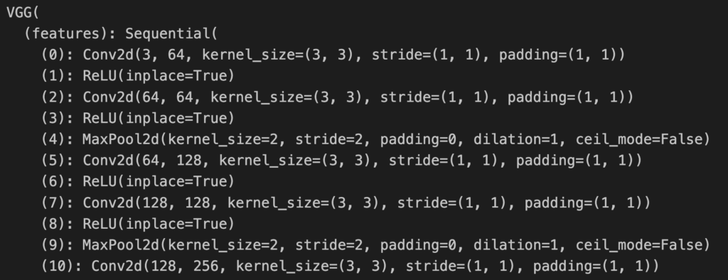
return top_catid[0]We load the pretrain VGG16 model (line 2), move it to a GPU (lines 5-8) and set it to evaluation mode (line 11). You can see a snippet of the model output in Figure 3. These show 5 of 13 convolutional layers. There are also 3 fully connected layers that make up the 16 weighted layers in VGG16.
# Load the pre-trained model (e.g., VGG16)
model = models.vgg16(pretrained=True)

# Set the model to gpu
device = torch.device('mps' if torch.backends.mps.is_built()
                      else 'cuda' if torch.cuda.is_available()
                      else 'cpu')
model.to(device)

# Set the model to evaluation mode
model.eval()
The names you see in Figure 3 are important. Later, we will use them to reference specific layers in the network and display their gradients. For example, features.5 is the name of the 3rd convolutional layer.
We display our example image that will be used as input into the model (lines 2-6). You can see this in Figure 4. I took this on a recent trip to Japan. ImageNet has no class for sushi so it will be interesting to see what prediction it makes.
# Load a sample image
img_path = "sushi.png"
img = Image.open(img_path).convert("RGB")

plt.imshow(img)
plt.axis("off")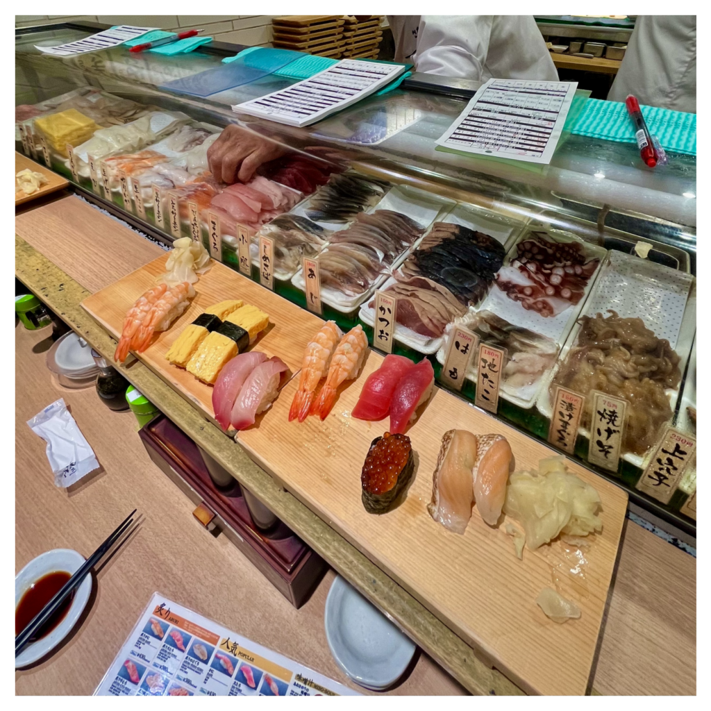
Let’s get a prediction for this image and visualise its gradients using standard backpropagation. These will be useful to compare to the GBP gradients we get later.
Standard backpropagation
We start by processing our image (line 2) and moving it to a GPU (line 3). The tensor gradients are stored and can be accumulated or overridden. So, to avoid doing this unintentionally, it is good practice to clone the input tensor (line 6). Gradients are typically used to update model parameters and not calculated for the input image. So, we must also enable gradient tracking for the image tensor (line 7).
# Preprocess the image
original_img_tensor = preprocess_image(img_path)
original_img_tensor = original_img_tensor.to(device)

# Clone tensor to avoid in-place operations
img_tensor = original_img_tensor.clone()
img_tensor.requires_grad_() # Enable gradient tracking
We now do a forward pass to get a prediction for the input image (line 1). We then display the output (line 4). In Figure 5, you can see the top 5 predictions. Given all the possible classes, a grocery store seems like a reasonable prediction.
predictions = model(img_tensor)

# Decode the output
display_output(predictions)
Before we do a backward pass it is good practice to reset the model’s gradients (line 2). Again, this is because gradients can be accumulated when making multiple backward passes. We want to find the gradients of the logit with the highest score. We select this (line 5) and use it to perform a backward pass (line 8). This will calculate the gradients of this logit w.r.t. to activations of intermediate layers and input values.
# Reset gradients
model.zero_grad()

# Select the class with the highest score
target_class = predictions.argmax()

# Compute gradients w.r.t to logit by performing backward pass
predictions[:, target_class].backward()
The backward pass will update img_tensor with the gradients. This allows us to select the gradients from the tensor (line 1). We also detach the gradients so that any operations do not impact the original tensor (line 1). Outputting the shape gives us dimensions (1, 3, 244, 244). We have a batch size of 1 and gradients for the 3 RGB channels in our input image. These results give us \( (\frac{\partial y_c}{\partial X}) \) or, in other words, how a small change in each pixel of the input image would affect the target logit’s value.
standard_backprop_grads = img_tensor.grad.detach().cpu().numpy() #do not detach the gradient
print(standard_backprop_grads.shape) # (1, 3, 224, 224)
We’ll use the process_grads function to help visualise the gradients. It gives a few options to help give clearer visualisation. It is common to use the ReLU activation function when visualising gradients for Guided Backpropagation. Although altering the ReLU functions in the network will suppress negative gradients, they can still be introduced in previous layers. For example, by the convolutional layer before the last ReLU.
def process_grads(grads_in,activation="None",skew=True,normalize=True,greyscale=False):
"""
Process the gradients for visualization.
Parameters:
grads (np.array): Gradients to be processed.
activation (str): Activation function to be applied to the gradients. Options: "relu", "abs".
skew (bool): Whether to skew the gradients.
Returns:
np.array: Processed gradients.
"""
# Copy the gradients so we do not change the original
grads = np.copy(grads_in)
# Transpose so the gradients have the same dimensions as an image
if len(grads.shape) >= 3:
grads = np.transpose(grads, (1, 2, 0))
# Relu to only view positive gradients
if activation == "relu":
grads = np.maximum(0, grads)
# Abs to give equal weight to positive and negative
elif activation == "abs":
grads = np.abs(grads)
# View both positive and negative
else:
grads = grads
# Normalize so they are between 0 and 1
# We add small value for the case of empty feature maps
if normalize:
grads -= np.min(grads)
grads /= (np.max(grads)+1e-9)
# Skew so we give more weight to small gradients
if skew:
grads = np.sqrt(grads)
# Convert to greyscale by averging across all channels
if greyscale:
grads = np.mean(grads, axis=-1)
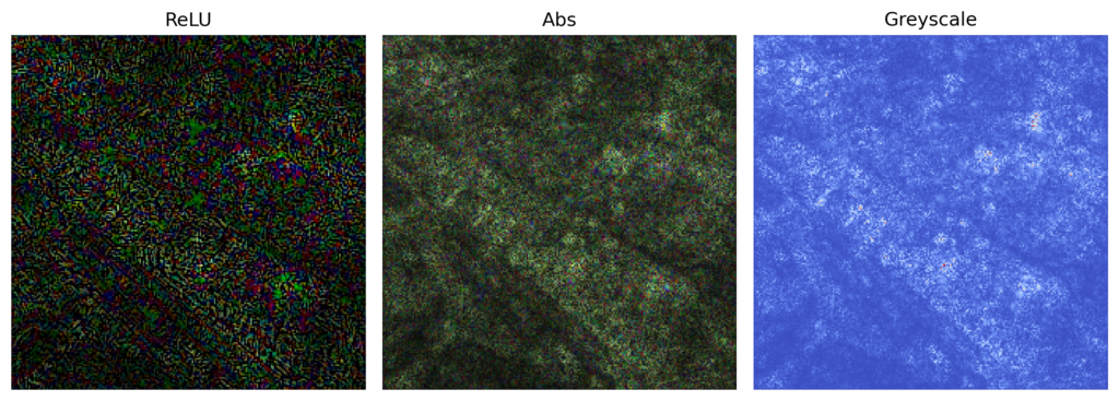
return gradsWe use this function to display our gradients in a few different ways. You can see these in Figure 6. In each case, the gradients are normalised and skewed. The latter operation means that smaller gradients are given more weight in the visualisation. This reduces the impact of larger outlier gradients.
grads = standard_backprop_grads[0]

# Process the gradients
relu_grads = process_grads(grads,activation="relu")
abs_grads = process_grads(grads,activation="abs")
grey_grads = process_grads(grads,activation="abs",greyscale=True,skew=False)

fig, ax = plt.subplots(1, 3, figsize=(10, 5))

# Display as an image
im0 = ax[0].imshow(relu_grads)
ax[0].title.set_text("ReLU")

im1 = ax[1].imshow(abs_grads)
ax[1].title.set_text("Abs")

im2 = ax[2].imshow(grey_grads, cmap="coolwarm")
ax[2].title.set_text("Greyscale")

for a in ax:
    a.axis("off")
With standard backpropagation, you can already see some important regions. It looks like the table and glass are contributing to the prediction. However, there is a lot of noise in the output. Let’s see how GBP can clean things up.
PyTorch hooks for guided backpropagation
To implement Guided Backpropagation, we will use PyTorch hooks to change how gradients flow through the network. We also use them to save gradients from intermediate layers. In a later section, we will use them to save activations from intermediate layers. Before that, we must replace the ReLU activation functions in the network.
Our VGG16 network has been created using ReLU with inplace=True. These modify tensors in memory, so the original values are lost. That is, tensors used as input are overwritten by the activation. This can lead to problems when applying hooks, as we may need the original input. While PyTorch allows registering hooks on in-place operations, it may cause runtime errors during backpropagation because the computational graph expects unmodified activations for gradient computation.
We use the code below to replace all ReLU activations with inplace=False ones. This will not impact the output of the model, but it will increase its memory usage. It is important to apply this code before registering any hooks on the ReLU functions. Otherwise, the hooks will be removed.
# Replace all in-place ReLU activations with out-of-place ones
def replace_relu(model):

    for name, child in model.named_children():
        if isinstance(child, torch.nn.ReLU):
            setattr(model, name, torch.nn.ReLU(inplace=False))
            print(f"Replacing ReLU activation in layer: {name}")
        else:
            replace_relu(child)  # Recursively apply to submodules

# Apply the modification to the VGG16 model
replace_relu(model)
The hook below will be applied to the ReLU functions in the network. By default, all backwards hook functions will have three parameters:
- module: the different components or layers of a neural network.
- grad_in: the gradients of the input into the module
- grad_out: the gradients of the output of the module
We also have an additional parameter, layer_name, which is the name of the module. These will be the same as those we saw in the model summary in Figure 3.
Going back to Figures 1 and 2, it is grad_in that is passed to the previous layer in the network during the backward pass. This is why we modify grad_in with the ReLU_hook function (line 17). We do this by replacing all negative gradients with a value of 0 (line 19) and keeping any empty gradients (line 21). Finally, we return the modified gradients (line 26). This will be the new grad_in pass to previous layers. It must be formatted as a tuple for cases where the layer has multiple inputs.
The code will also store the modified gradients (line 24). These will be used when we visualise the gradients of intermediate layers. We detach these from the computational graph so that visualising them does not impact the network (line 24). These gradients will be stored in the gradients dictionary (line 2) with the layer’s name as the key (line 24).
# Dictionary to store gradients
gradients = {}

def relu_hook(module, grad_in, grad_out, layer_name):
    """
    Guided Backpropagation Hook: Allows only positive gradients to backpropagate.

    Parameters:
        module (nn.Module): The module where the hook is applied.
        grad_in (tuple of Tensors): Gradients w.r.t. the input of the module.
        grad_out (tuple of Tensors): Gradients w.r.t. the output of the module.
        layer_name (str): Name of the module.
    """

    modified_grad = []  # Create a list to store modified gradients

    for g in grad_in:
        if g is not None:
            modified_grad.append(torch.clamp(g, min=0.0))  # Keep only positive gradients
        else:
            modified_grad.append(None)  # Preserve any None values in grad_in

    # Save gradients
    gradients[layer_name] = modified_grad[0].detach().cpu().numpy().squeeze()

    return tuple(modified_grad)
We then iterate through all modules in the layer (line 2). If the module is a ReLU action function, we register the ReLU_hook function(lines 5-11). We use the register_backward_hook function as we want the hook to be used during the backward pass (line 6). When doing this, we use a lambda function as we must also pass the layer’s name as a parameter (lines 6-10). If a hook uses only the default parameters, you can simply pass the function’s name to the register_backward_hook function.
# Register the hook for all layers
for name, layer in model.named_modules():

    # Update the hook for ReLU layers
    if isinstance(layer, torch.nn.ReLU):
        layer.register_backward_hook(lambda m,
                                     gi,
                                     go,
                                     n=name:
                                     relu_hook(m, gi, go, n))
        print(f"Relu hook registered for {name}")
Guided backpropagation for target logit
With the hooks in place, we can apply Guided Backpropagation. We’ll start by finding the gradients of a target logit w.r.t. to the input \( \left( \frac{\partial y_c}{\partial X} \right) \). To do this, we follow the same process as we did for standard backprop (lines 1-13). Except now, during the backward pass (line 13), the ReLU_hook will be applied and only positive gradients will be propagated at the ReLU activation functions. Later, we will also use the gradients it saves to the gradients dictionary.
# Reset gradients
img_tensor = original_img_tensor.clone()
img_tensor.requires_grad_()
model.zero_grad()
# Get the model's prediction (with gradient calculation)
predictions = model(img_tensor)
# Select the class with the highest score
target_class = predictions.argmax()
# Compute gradients w.r.t to logit by performing backward pass
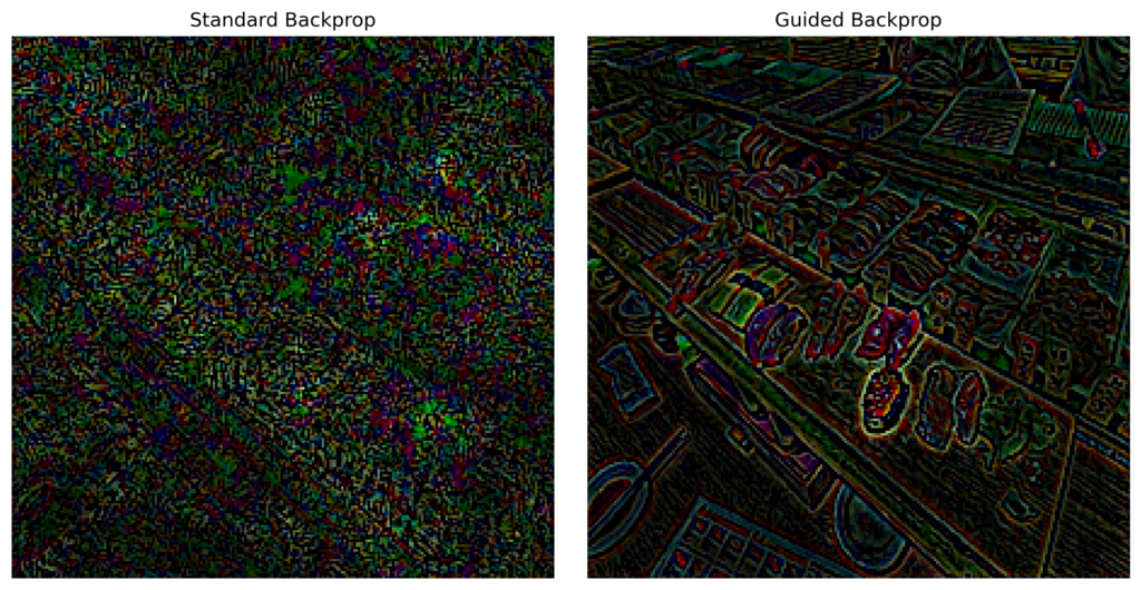
predictions[:, target_class].backward()We get the GBP gradients from the image tensor (line 2). We process them using the ReLU function to remove any negative gradients introduced by the first convolutional layer (line 3). We then plot these alongside the gradients from standard backprop that we got earlier (lines 8-15). You can see the result in Figure 7.
# Get the image gradients
grads = img_tensor.grad.detach().cpu().numpy().squeeze()
grads = process_grads(grads,activation="relu")

fig,ax = plt.subplots(1,2,figsize=(10,5))

# Display the gradients
ax[0].imshow(relu_grads)
ax[0].title.set_text("Standard Backprop")

ax[1].imshow(grads)
ax[1].title.set_text("Guided Backprop")

for a in ax:
    a.axis("off")
You’ll notice that GBP has produced a much clearer interpretation. Looking at the standard backprop, we may be able to understand important regions of the image. In comparison, with GBP we can see edges and objects that are important. Intuitively, the different foods appear to be contributing to the grocery store prediction.
The above example shows how GBP can be used to explain an individual prediction of the model. That is we can understand which features in the input image are important. This insight can help debug incorrect predictions. We can also go further with GBP to understand the features extracted at the internal layers.
Guided backpropagation from intermediate layers in a neural network
# Gradients from the first layer
layer = 'features.1'

# Get gradients for all feature map in layer
layer_grads = gradients[layer]
print(layer_grads.shape)

# Select a random feature map
i = np.random.randint(0, layer_grads.shape[0])
feature_map_grads = layer_grads[i]

# Processing the gradients
feature_map_grads = process_grads(feature_map_grads)

# Display the gradients
plt.imshow(feature_map_grads, cmap="coolwarm")
plt.axis("off")
As mentioned, we saved the gradients for intermediate layers obtained during backpropagation. Above we are visualizing \(\frac{\partial{y_c}}{\partial X} \) where X is the input. With the intermediate layers we want to \(\frac{\partial{y_c}}{\partial A}\). That is the gradients of the target logit w.r.t. activations of a feature map A. Specifically, as we saw in Figure 2, the ReLU_hook saves the modified gradients of the input into the ReLU activation layers. These are the positive gradients passed to previous layers in the network.
The gradients stored at each ReLU layer will have the same number of channels as the kernels in the previous convolutional layer. Going back to the model output in Figure 2, we saw that features.0 was a convolutional layer with 64 kernels. This means the gradients saved at features.1, the next ReLU layer, will have 64 channels.
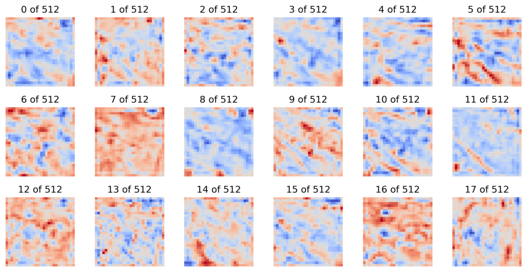
Considering this, we use the code below to visualise some random feature maps from 4 different layers in the network. We start with the first layer and make our way down the network to deeper layers (line 3). When processing the gradients, we do not need to use the ReLU activation (line 12). The gradients will already be positive because of the ReLU_hook. You can see the output in Figure 8.
fig, ax = plt.subplots(4, 5, figsize=(15, 15))

for i,layer in enumerate(['features.1','features.6','features.13','features.22']):
    layer_grads = gradients[layer]
    print(f"{layer}: {layer_grads.shape}")

    for j in range(5):
        n_features = layer_grads.shape[0]
        r = np.random.randint(0, n_features)

        feature_map_grads = layer_grads[r]
        feature_map_grads = process_grads(feature_map_grads)

        ax[i, j].imshow(feature_map_grads, cmap="coolwarm")

        ax[i, j].set_title(f"{r} of {n_features}")
        ax[i, j].set_xticks([])
        ax[i, j].set_yticks([])

    ax[i, 0].set_ylabel(f"{layer}", fontsize=15)

plt.tight_layout()
Looking at feature maps like these, we can gain a deeper understanding of how the network works. Like most CNNs, earlier layers detect basic patterns like edges and textures. Deeper layers detect more abstract features like object parts. The deepest layers detect abstract, global features that represent entire objects or semantic meaning. GBP helps in visualising this behaviour by ensuring that only the patterns that positively contributed to the prediction are highlighted.

These kinds of insights go beyond understanding the nature of CNNs. They can actually be used to improve the performance or efficiency of a model. For example, [2] introduced a method called deconvolution, which is the precursor GBP. They used the approach to visualise the first and second layers of a network, identify problems and adjust the convolutional layer’s filter size and stride to correct them.
Going back to the general nature of CNNs, in Figure 8, we can clearly see that spatial information is preserved in earlier layers. That is for features.1 we can see different edges and textures in the same location as the objects in the input image. What is not so obvious is that this spatial information is preserved even in the deeper layers like features.22. We’ll prove this using our next approach.
Guided backpropagation starting from activations in an intermediate layer of a neural network
Until now, we have visualised gradients for an output logit, \(y_c\). We can also apply Guided Backpropagation to visualise the gradients of the output of any layer in the network. We’ll see how by finding the gradients of an element in the feature maps from one of the convolutional layers \(\left( \frac{\partial y_c}{\partial A_{ij}} \right)\).
To start, we will need to store the output of all the convolutional layers. To do this, we create a new hook function, act_hook_fn that will store the output of a layer to the activations dictionary. An important difference is we do not detach the output (line 15). We need it to be connected to the computation graph as we will do backward passes starting at different elements in these activations.
# Dictionary to store activations
activations = {}

def act_hook_fn(module, input, output, layer_name):
    """
    Hook function to store activations of a layer.

    Parameters:
        module (nn.Module): The module where the hook is applied.
        input (tuple of Tensors): Incoming data to the layer.
        output (Tensor): Outgoing data from the layer.
        layer_name (str): The name of the layer.
    """
    # Store the activations as tensors
    activations[layer_name] = output.clone()
    print(f"Activation stored for {layer_name}")
We apply this hook to every convolutional layer (lines 2-5). If we look back at Figure 1, this means we will be saving the “output” feature maps from the forward pass. When registering the hook, it is important to now use the register_forward_hook function. This is because we want to save the output from the forward pass.
# Register hooks on all convolutional layers
for name, layer in model.named_modules():
    if isinstance(layer, torch.nn.Conv2d):
        layer.register_forward_hook(lambda m, i, o, n=name: act_hook_fn(m, i, o, n))
        print(f"Forward hook registered for {name}")
We make a prediction using our sample image (lines 2-7). This is the forward pass and so the activations for all convolutional layers will be saved.
# Reset gradients
img_tensor = original_img_tensor.clone()
img_tensor.requires_grad_()
model.zero_grad()

# Perform a forward pass
predictions = model(img_tensor)
We can see this when we select the activations for the convolutional layer, features.21 (line 10). The shape of the layer (512, 28, 28). In other words, we have 512 feature maps and each map has 28 by 28 elements.
# Get the activations of the conv layers
layer_act = activations['features.21'][0]
print(layer_act.shape) # (512, 28, 28)
We visualise the first 18 feature maps from this layer (lines 1-3). You can see these in Figure 9. Unlike the gradients, these values can be both positive and negative, depending on what features are extracted by each map.
# Plot the activations
fig, ax = plt.subplots(3, 6, figsize=(10, 5))

for i, act in enumerate(layer_act[0:18]):

    act_copy = act.clone().detach().cpu().numpy()
    act_copy = process_grads(act_copy,skew= False)

    ax[i // 6, i % 6].imshow(act_copy, cmap="coolwarm")
    ax[i // 6, i % 6].set_title(f"{i} of {layer_act.shape[0]}")
    ax[i // 6, i % 6].axis("off")

plt.tight_layout()
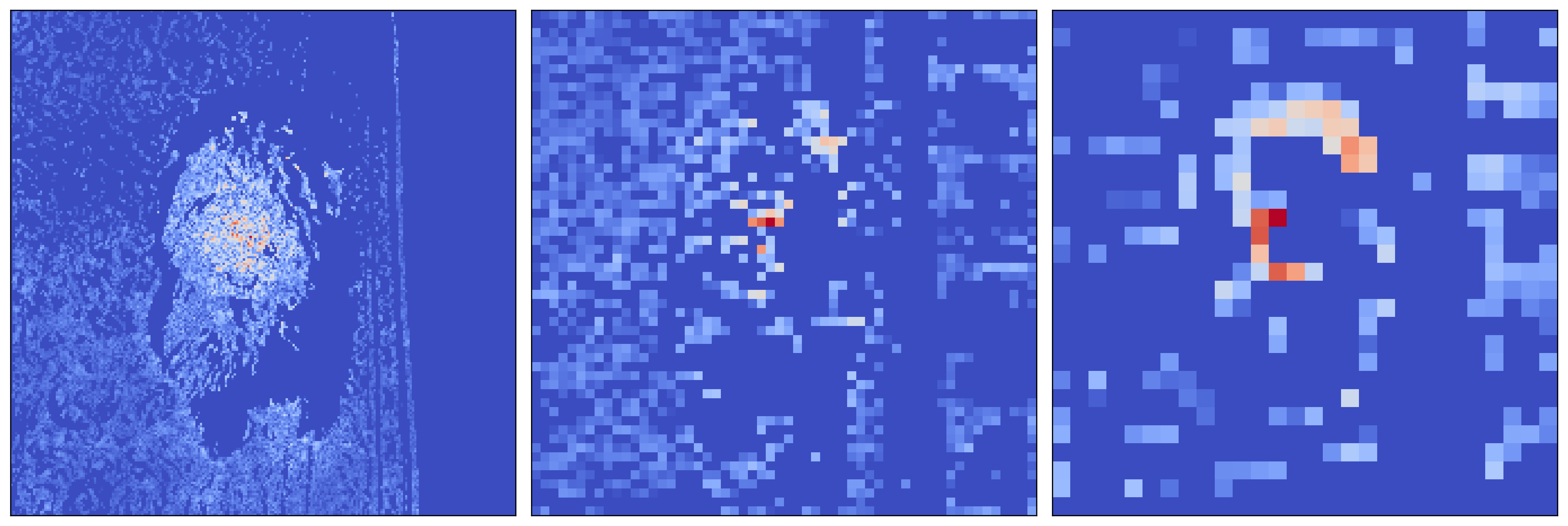
Now let’s do a backward pass starting at one of these activations (line 2). Specifically, we have used the element at position (14,14) from the first feature map. This is a point that is roughly in the middle of the (28, 28) map. When we do this, our backwards hook still applies, so only positive gradients are propagated. Although we won’t use them, you will also see that the gradients for intermediate layers, starting at this layer, are saved.
# Compute gradients w.r.t element of the feature map
layer_act[0][14,14].backward()
We visualise the gradients of the input image like we visualised them for the target logit (lines 2-6). Looking at Figure 10, you can see the features from the input image that are contributing positively to the activation from this element. Before we discuss this further, let’s repeat the same process for a few more elements in the feature map.
# Get the gradients of input image
grads = img_tensor.grad.detach().cpu().numpy().squeeze()
grads = process_grads(grads, activation="relu")

plt.imshow(grads)
plt.axis("off")
We do this for the positions given on line 1. These give elements from different corners of the feature map. You can see the gradients that contribute to each of these elements in Figure 11.
positions = [(5,5),(5,20),(20,5),(20,20)]

fig,ax = plt.subplots(2,2,figsize=(10,10))

for i, (x,y) in enumerate(positions):

    img_tensor = original_img_tensor.clone()
    img_tensor.requires_grad_()
    model.zero_grad() # Reset gradients

    predictions = model(img_tensor)

    # Get the activations of the conv layers
    layer_act = activations['features.21'][0]
    layer_act[0][x,y].backward()

    grads = img_tensor.grad.cpu().numpy().squeeze()
    grads = process_grads(grads,activation="relu")

    ax[i // 2, i % 2].imshow(grads)
    ax[i // 2, i % 2].set_title(f"Position: ({x},{y})")
    ax[i // 2, i % 2].axis("off")
Looking at Figure 11, you can see the different objects in the input that have contributed to the activated elements. These are made clear by GBP. Another thing you will have noticed is that the objects are in the same locations as the positions of the elements in the feature map. This demonstrates that, although the deeper feature maps contain more abstract features, they still retain spatial information from earlier layers.
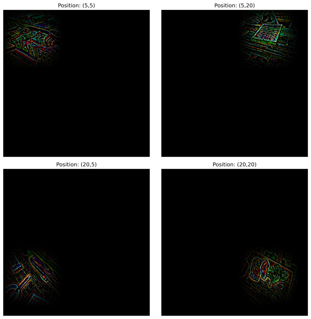
This property of CNNs is why our previous method, Grad-CAM, works so well. Those heatmaps were created by weighting the feature maps of the last convolutional layer in a network. If spatial information was not retained by that layer, then the heatmap would not identify important regions in the input.
Guided Backpropagation goes a long way in reducing noise in saliency maps. As we’ve seen, this can help explain individual predictions and the general behaviour of a network. Without RelU masking, the patterns we revealed here would not be as clear. However, there are still cases where Guided Backpropagation goes wrong.
In the next section, we will apply guided grad-cam. It is a method that combines Grad-CAM and Guided Backpropagation to harness the advantages of both methods. The result is even clearer saliency maps that highlight important features.
Challenge
Try to implement Grad-CAM without a package using only PyTorch hooks. You will need to apply both forwards and backwards hooks like in this lesson.
I hope you enjoyed this article! See the course page for more XAI courses. You can also find me on Bluesky | Threads | YouTube | Medium
References
[1] Jost Tobias Springenberg, Alexey Dosovitskiy, Thomas Brox, and Martin Riedmiller. Striving for simplicity: The all convolutional net. arXiv preprint arXiv:1412.6806, 2014.
[2] MD Zeiler. Visualizing and understanding convolutional networks. In European conference on computer vision/arXiv, volume 1311, 2014.
Get the paid version of the course. This will give you access to the course eBook, certificate and all the videos ad free.