Input X Gradients
Why multiplying by gradients gives us sharper saliency maps (and why the interpretation is dodgy)

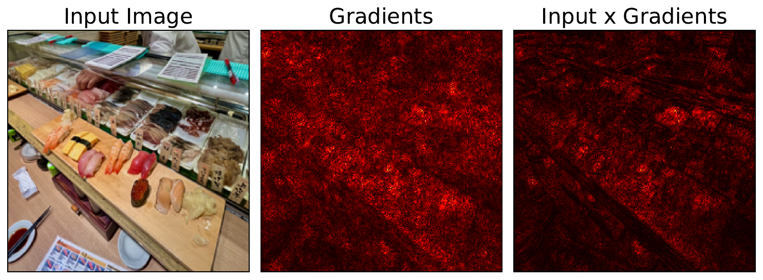
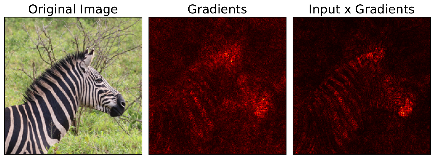
We start where we left off on Vanilla Gradients. We take the gradients we calculated in that section and multiply them by the input image (line 7). A key point is that we are using the same input as what is provided to the model (line 1). This has been normalised using the standard ImageNet mean and deviation. We then visualise the gradients and input X gradients in the same way (line 10-11). You can see the output from our sushi image in Figure 1. There is also another example using a different input image (Zebra image) in Figure 2.

input = original_img_tensor.clone()
input = input.detach().cpu().numpy()

gradients = standard_backprop_grads.copy()

# Input times gradients
attribution = input * gradients

# Process attributions
gradients = process_attributions(gradients, activation="abs", skew=0.8, colormap="hot")
attribution = process_attributions(attribution, activation="abs", skew=0.8,  colormap="hot")

You can see that in both images, when we multiply by the input, the saliency map becomes sharper. This effect is more prominent with the second image, where the zebra's stripes are now clearly visible. However, we need to keep in mind that the interpretation of these saliency maps can be dubious when it comes to image data. To understand this, we can compare it to the interpretation when applied to tabular data.

Interpreting Input X Gradients: Sensitivity-based vs contribution-based attributions

Input X Gradients is inherently a heuristic. However, researchers have suggested that multiplying by input does more than just improve the sharpness of saliency maps. They change the nature of the explanation from a Sensitivity-based one to a contribution-based one [2]. This takes us back to the definition we introduced in the taxonomy lesson:

• Sensitivity-based (a.k.a. local) attributions: describe how the output of the network changes for infinitesimally small perturbations around the original input.
• Contribution-based (a.k.a. global) attributions: describe the marginal effect of a feature on the output with respect to a baseline.

To understand this, let's take a simple linear model:

\[
y = 100 x_{1} + 5x_{2}+ 1000
\]

Here, a maximum loan amount (\(y\)) is a function of a person's age (\(x_1\)) and income (\(x_2\)). Suppose we have a customer who is 30 years old and makes \euro50,000 a year. We can try to explain the prediction using gradients:

\[
\frac{\partial y}{\partial x_1 } = 100
\]

\[
\frac{\partial y}{\partial x_2 } = 5
\]

These tell us how much the predicted loan amount will change if we make small changes to the customer's features. That is the sensitivity of the output to the input. However, if we used these values, we would incorrectly conclude that the contribution of age is 20 times higher than income. Instead, let's multiply the gradients by the input:

\[
x_1\frac{\partial y}{\partial x_1 } = 30*100 = 3000
\]

\[
x_2\frac{\partial y}{\partial x_2 } = 50000*5 = 250000
\]

Now we see that the importance of income is significantly higher. For the linear models, the interpretation of this is straightforward. We are essentially multiplying feature values by their corresponding parameters in the model. For each feature, this gives us the marginal contribution compared to baseline values of 0. For more complex, non-linear models trained on tabular data, the intuition is similar.

The difference is that we now multiply the gradient of a feature (i.e. sensitivity to change) by the feature's value (i.e. how much it deviates from a baseline of 0). However, the interpretation only makes sense when a feature has an approximately linear relationship over that range. It also only makes sense because with tabular data, the values of features are typically meaningful. For example, a higher value for \(x_2\) means that a customer has more income.

When it comes to image data, this interpretation breaks down. It is probably not safe to assume pixel values have a linear relationship with the model's output. The values of pixels also have arbitrary encodings. For example, as seen in Figure 3, if we scaled images using min-max (dividing by 255), then darker pixels would have lower values, with a value of 0 for black pixels. In our case, we are using the standard ImageNet normalization values, and so dark pixels will have large negative values and light pixels will have large positive values. However, this does not mean these pixels are less important to the prediction.

Ultimately, for image data, when multiplying by the input, we may produce saliency maps that are biased towards lighter or darker pixels. Although the Input X Gradients method can produce a more visually pleasing saliency map, it may simply be appropriating the structure from the input image. However, this is not true for all gradient-based methods that use a baseline. We will see this when discussing Integrated Gradients, the contribution-based interpretation is valid. The difference is that this method considers the gradients of many images along a path from the baseline to the input image. For now, we will move on to some other heuristic-based methods.

Challenge

Apply the Input X Gradient method to a model where the training data has been scaled his min-max or by dividing by 255. What do you notice about the saliency of dark pixels?

References

- Shrikumar, Avanti, Greenside, Peyton, Shcherbina, Anna, et al. (2016). Not just a black box: Learning important features through propagating activation differences. arXiv preprint arXiv:1605.01713.
- Ancona, Marco, Ceolini, Enea, Oztireli, Cengiz, et al. (2017). Towards better understanding of gradient-based attribution methods for deep neural networks. arXiv preprint arXiv:1711.06104.
Get the paid version of the course. This will give you access to the course eBook, certificate and all the videos ad free.