LIME for Computer Vision
How superpixels, lasso regression, and kernel weighting combine to create local XAI explanations

The LIME algorithm

Machine learning models are complex functions. The idea behind LIME is that this complexity falls away if we zoom into the feature space in the area around an instance. The function is much simpler or even linear. This allows us to understand how predictions are made in this area using simple surrogate models.

Now, there is a lot of choice around how we build such a surrogate model. We discuss the most important ones below. First, let's summarize the steps taken by the LIME algorithm:

1. Select the instance you want to explain.
2. Generate samples by permuting feature values.
3. Assign a weight to each of the samples based on how far they are from the instance.
4. Make predictions on these permutations using the original black-box model.
5. Train a surrogate model using the weighted samples and predictions as the target variable.
6. Interpret the surrogate model.

Creating features with superpixels

LIME requires us to create a new dataset that is used to train a surrogate model. For tabular data, we sample feature values from their distributions in the training data. For continuous features, we sample from the normal distribution with the same mean and standard deviation as the feature. For categorical features, we randomly select categories based on their observed proportions.

For image data, this approach fails for two reasons. First, pixels are spatially dependent, so sampling them independently from statistical distributions destroys meaningful visual structure. Just think about whether it would make sense to replace pixels with ones in the same position in other images. Second, treating each pixel as a separate feature creates an unmanageable number of highly correlated features. This can lead to unstable coefficient estimates for linear models.

Instead, as seen in Figure 1, we divide the image into superpixels. These are groups of connected pixels in an image that share similar visual characteristics, such as color, brightness, or texture. They are created using superpixel algorithms like SLIC [1] and Felzenszwalb [2]. These superpixels yield the features used in our surrogate model. That is, the surrogate model will have the same number of features as there are superpixels. Interpreting it will show us the importance of a group of pixels.

Permuting features

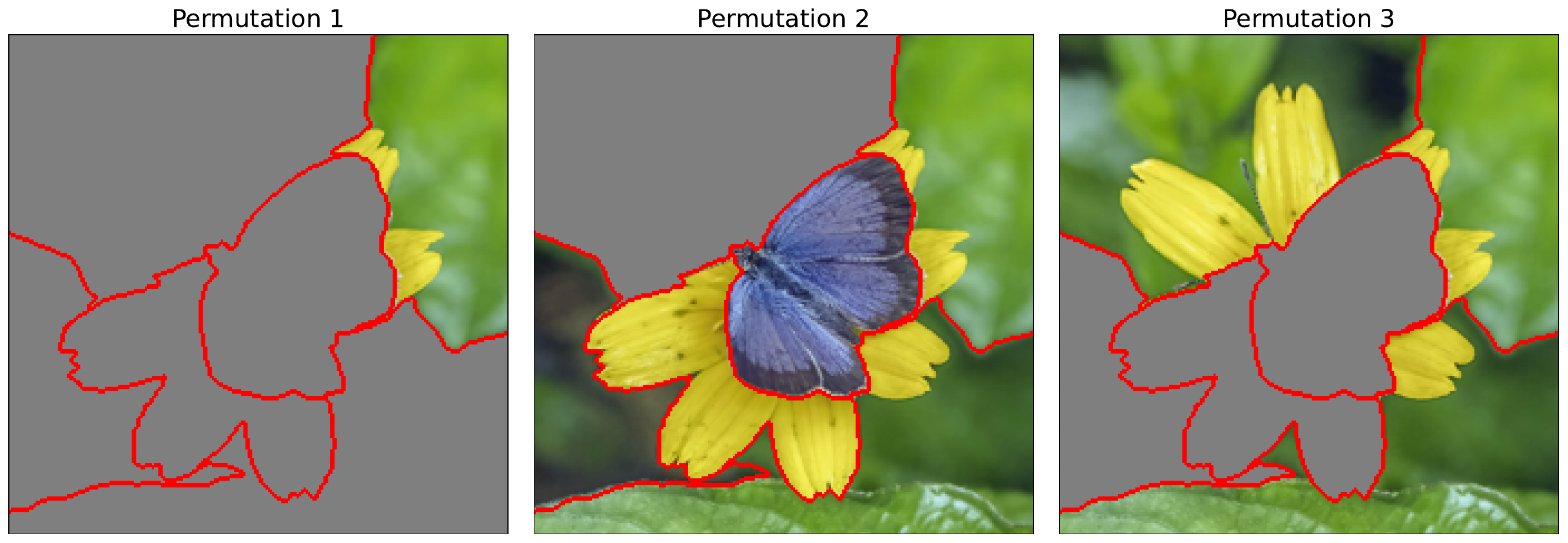
Like with occlusion, we permute the image using a baseline value. Specifically, we will randomly replace entire superpixels with the baseline value. You can see some examples in Figure 2. We do this many times, and by default, it is repeated 50 times in the Captum implementation. Each of these permutations becomes an input image used to generate the surrogate model dataset.

The surrogate model

The input for the surrogate model dataset is simplified by creating a binary vector based on whether a superpixel is permuted or not. As seen in Figure 3, the vector is given a value of 1 if the corresponding superpixel has the original values (i.e. is not permuted) and 0 if it has the baseline values (i.e. is permuted). In this case, we have 6 superpixels, and so we will be training a surrogate model with 6 binary features.

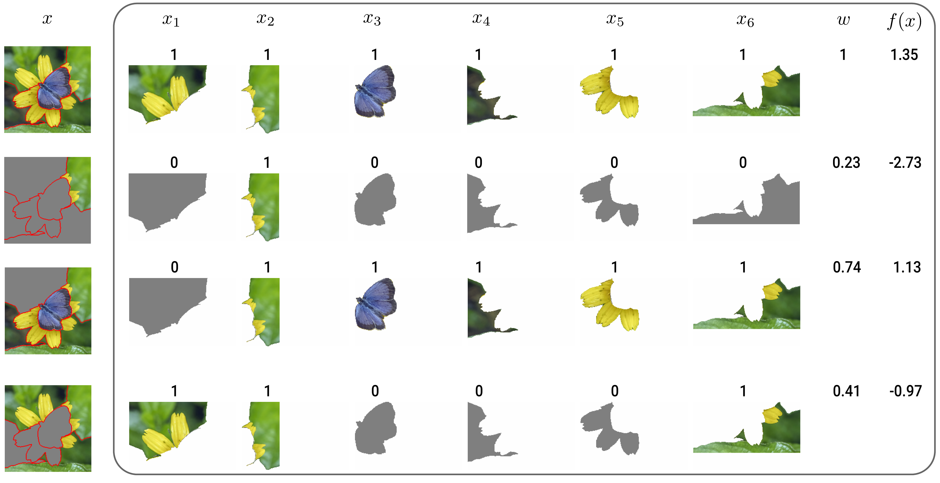
The output for the surrogate model dataset is obtained by feeding the permuted images into the black-box model. Specifically, we obtain the predicted logit for the class of interest, \(y_c\). We also obtain a weight for each instance based on how different the permuted image is from the original image. These outputs (\(y_c\)), inputs (\(x_i\)) and weights (\(w\)) are used to train the surrogate model.

When it comes to the algorithm used to develop the surrogate model, the default used by Captum is lasso regression. However, we can use other types of linear regression or even a decision tree. Keep in mind that the model must be inherently interpretable. For linear models, the coefficients give the importance of the corresponding features to the prediction we want to explain.

Weighting samples

With LIME, our goal is to understand how a model makes a prediction locally around a given instance. Yet, the above permutation process will produce instances that are different from that image. This is why we weight the samples based on their distance from the instance. However, this interpretation may be more appropriate for tabular data where we are generating features across the entire feature range.

A more relevant concern is that images with permuted superpixels are unlike any a model was trained on. These out-of-distribution samples can result in unexpected explanations [3]. This problem may be worse when we permute a large number of superpixels. The weighting could therefore help reduce this effect by reducing the contribution of these samples. In other words, for image data, the weights can be thought of as an indication of certainty in the black box model prediction.

To create weights, LIME uses the Gaussian kernel seen in Equation 1. Where \(D(x,x')\) is a distance function between the original instance \(x\) and perturbed sample \(x'\). For larger distances, the kernel will give a value closer to 0. For smaller distances, it will give a value closer to 1, with a value of 1 when the distance is 0. The rate at which the weight decreases with distance is controlled by the kernel width, \(\sigma^2\).

\[ K(x, x') = \exp(-\frac{D(x, x')^2}{\sigma^2}) \]

We have a choice when it comes to the distance function. The default used by Captum is the cosine distance:

\[ D_{cos}(x, x') = 1 - \frac{x \cdot x'}{\|x\|_2 \|x'\|_2} = 1 - \frac{\sum_{i=1}^{n} x_i x'_i}{\sqrt{\sum_{i=1}^{n} x_i^2} \sqrt{\sum_{i=1}^{n} x_i'^2}} \]

The function suggested for image data in the LIME paper is the Euclidean distance:

\[ D_{L2}(x, x') = \sqrt{\sum\nolimits_{i=1}^{n} \left(x_i - x'_i\right)^2} = \|x - x'\|_2 \]

These are applied to the binary vectors obtained from the original and permuted images. To demonstrate how these are used, we will apply them to the first two rows from Figure 3. The two vectors are \(x=[1,1,1,1,1,1]\) and \(x'=[0,1,0,0,0,0]\):

\[ x \cdot x' = (1)(0) + (1)(1) + (1)(0) + (1)(0) + (1)(0) + (1)(0) = 1 \]

\[ \|x\|_2 = \sqrt{1^2 + 1^2 + 1^2 + 1^2 + 1^2 + 1^2} = \sqrt{6} \]

\[ \|x'\|_2 = \sqrt{0^2 + 1^2 + 0^2 + 0^2 + 0^2 + 0^2} = \sqrt{1} = 1 \]

\[ D_{cos}(x, x') = 1 - \frac{1}{\sqrt{6} \cdot \sqrt{1}} \approx 0.59 \]

\[ \begin{aligned} D_{L2}(x, x') & = \sqrt{(1-0)^2 + (1-1)^2 + (1-0)^2 + (1-0)^2 + (1-0)^2 + (1-0)^2} \\ & = \sqrt{5} \\ & \approx 2.24 \end{aligned} \]

In terms of kernel width, the default used by Captum is a value of 1. This is likely as they use cosine as the default distance, which already produces distance values between 0 and 1. For Euclidean distance, in the LIME paper, they found that setting \(\sigma = 0.75 \times \sqrt{\text{number_of_features}}\) produced good results. For image data, this will be \(0.75 \times \sqrt{\text{number_of_superpixels}}\). This is potentially as with the Euclidean distance, the values will tend to be larger the more features you have.

So, as we have seen, there is a lot of choice when it comes to implementing LIME. We need to select the superpixel algorithm, the number of superpixels, the distance function, kernel width and even the algorithm used for the surrogate model. All of these choices may seem like a good thing. However, it leads to one of LIME's biggest weaknesses.

The limitations of LIME

Inconsistent explanations

The flexibility when implementing LIME can lead us to different explanations using the same method. It also opens us up to a form of p-hacking, as we can manipulate the variables until we get the explanations we want. Ultimately, there is no way of telling which explanation is correct or which is due to random chance. This leads to uncertainty around the reliability and faithfulness of LIME saliency maps. A problem which is made worse by the unrealistic assumptions of the method.

Out-of-distribution samples

As mentioned, LIME's perturbation process creates samples that differ significantly from the training data. We are assuming that model output behaves reliably over these samples. However, when large portions of an image are masked and replaced with a baseline (e.g., grey pixels), the resulting sample no longer resembles natural images. While LIME's distance-based weighting reduces the influence of these out-of-distribution samples, explanations can still be contaminated by unreliable predictions.

Assumption of local linearity

The core assumption of LIME is that the model can be approximated by a linear function in a small neighbourhood around the input. This can be true even for CNNs, which have many nonlinear components. The perturbation strategy must just make changes that are small enough so that we do not change activation states (e.g. ReLU changing from 0 to positive). The problem is that this is most likely not achieved with the way LIME is applied to image data.

The changes we make to images are significant. Replacing even one superpixel with the baseline may move the input out of the small linear neighbourhood. So, even if the assumption of local linearity is true, in practice it is violated by the perturbation strategy. This means we may end up with unreliable attributions even if the previous limitation is not a problem and the model behaves smoothly on perturbed samples.

We explore this last assumption in more depth when talking about SHAP. For now, let's move on to applying LIME. We'll be doing this using the default version of LIME as well as testing out different distance metrics. Just remember that in all cases, LIME can produce explanations that misrepresent how the model actually processes visual information.

Applying LIME with Captum

We start with our imports. We'll be using the SLIC superpixel algorithm (line 8) to help create our features. We also have the Lime function from Captum (line 13).

import matplotlib.pyplot as plt 
import numpy as np
import pandas as pd

from PIL import Image

from skimage.segmentation import mark_boundaries
from skimage.segmentation import slic

import torch
from torchvision import models

from captum.attr import Lime

# Helper functions
import sys
sys.path.append('../')

from utils.visualise import display_imagenet_output
from utils.datasets import preprocess_imagenet_image

Load model and input image

For our model, we'll use EfficientNet B0 pretrained on ImageNet. To help, we have the two functions below. These will also be used later in the course whenever we use ImageNet models.

The first function, preprocess_imagenet_image, will correctly format an image for input into the model. The normalization values used are the mean and standard deviation of the images in ImageNet. The code for this function is found in the dataset.py file in the utils folder.

def preprocess_imagenet_image(img_path):

    """Load and preprocess images for PyTorch models."""

    img = Image.open(img_path).convert("RGB")

    #Transforms used by imagenet models
    transform = transforms.Compose([
        transforms.Resize((224, 224)),
        transforms.ToTensor(),
        transforms.Normalize(mean=[0.485, 0.456, 0.406], std=[0.229, 0.224, 0.225]),
    ])

    return transform(img).unsqueeze(0)

ImageNet has many classes. The second function, display_imagenet_output, will format the output of the model so we display the classes with the highest predicted probabilities. This can be found in the visualise.py file in the utils folder.

def display_imagenet_output(output,n=5):

    """Display the top n categories predicted by the model."""

    # Download the categories
    url = "https://raw.githubusercontent.com/pytorch/hub/master/imagenet_classes.txt"
    urllib.request.urlretrieve(url, "imagenet_classes.txt")

    with open("imagenet_classes.txt", "r") as f:
        categories = [s.strip() for s in f.readlines()]

    # Show top categories per image
    probabilities = torch.nn.functional.softmax(output[0], dim=0)
    top_prob, top_catid = torch.topk(probabilities, n)

    for i in range(top_prob.size(0)):
        print(categories[top_catid[i]], top_prob[i].item())

    return top_catid[0]

We load the pretrained EfficientNet model (line 2), move it to a GPU (lines 5-8) and set it to evaluation mode (line 11). As LIME is model agnostic we are not particularly interested in the model architecture. The process we use here will be the same for any ImageNet model.

# Load the pre-trained model (e.g., efficientnet_b0)
model = models.efficientnet_b0(weights=models.EfficientNet_B0_Weights.IMAGENET1K_V1)

# Set the model to gpu
device = torch.device('mps' if torch.backends.mps.is_built() 
                      else 'cuda' if torch.cuda.is_available() 
                      else 'cpu')
model.to(device)

# Set the model to evaluation mode
model.eval()

You can download the example image for this lesson directly from Wikimedia Commons. Alternatively, as seen below, you can use the save_image function from the download.py file in the utils folder. Similar code is available for other lessons that use this image source.

# Download example image
import sys
sys.path.append('../')

from utils.download import save_image

url = "https://upload.wikimedia.org/wikipedia/commons/c/ce/Canis_latrans_%28Yosemite%2C_2009%29.jpg"
save_image(url, "coyote.png")

We load the example image of a coyote. We will display this later when calculating superpixels. For now, let's do a forward pass using this image.

# Load a sample image
img_path = "coyote.png"
img = Image.open(img_path).convert("RGB")

plt.imshow(img)
plt.title("Input Image")
plt.axis('off')

We start by processing our image (line 2) and moving it to a GPU (line 3). We now do a forward pass to get a prediction for the input image (line 6). We then display the output (line 9). Below, you can see the top 5 predictions.

# Preprocess the image
img_tensor = preprocess_imagenet_image(img_path)
img_tensor = img_tensor.to(device)

with torch.no_grad():   
    predictions = model(img_tensor)

# Decode the output
display_imagenet_output(predictions,n=5)

coyote 0.7475791573524475
timber wolf 0.14468714594841003
red wolf 0.016246657818555832
dingo 0.006272103637456894
white wolf 0.0049531529657542706

SLIC superpixel segmentation

The first step in applying LIME is to create features using superpixels. To do this, we use the SLIC algorithm (lines 3-6). We won't go into detail on how this works. Just know that it is used to create clusters of similar pixels based on their location and values. We have:

• n_segments (line 4): defines the number of initially, equally spaced cluster points
• compactness (line 5): determines how symmetrical the final cluster will be, with larger values being more symmetrical
• sigma (line 6): determines how much the image is blurred before the SLIC algorithm is applied

The specific values we chose here were determined using trial and error so that we got reasonable superpixels. Using the mark_boundaries function (line 9), we display the segments (line 11-15). You can see these in Figure 4. When we apply LIME, these superpixels will be selected randomly and then permuted by changing all the pixels within a superpixel to the baseline value.

# Apply SLIC superpixel segmentation
img = np.array(img)
segments = slic(img, 
                n_segments=20, 
                compactness=30,
                sigma=1)

# Visualize the segmentation results
boudaries = mark_boundaries(img, segments)

fig, ax = plt.subplots(1, 2, figsize=(12, 6))
ax[0].imshow(img)
ax[0].set_title("Input Image")
ax[1].imshow(boudaries)
ax[1].set_title("SLIC Segmentation")

Generating attribution

With our superpixels, we move on to applying LIME. To do this, we select the index of the target class (line 2). This is class 272 of ImageNet. We also format the superpixel segments as a tensor (line 7).

# Get the predicted class index
target_class = predictions.argmax().item()

print(f"Predicted class index: {target_class}")

# Format segments for LIME
feature_mask = torch.from_numpy(segments).unsqueeze(0).to(device)

We pass the model to the Lime function to create a LIME object. We use this to create an attribution by passing in the image tensor (line 3), the target class (line 4), our superpixel mask (line 5) and the number of samples (line 6). This latter parameter determines how many random permutations are made when generating the attribution.

# Get LIME attribution
lime = Lime(model)
attr = lime.attribute(img_tensor, 
                        target=target_class, 
                        feature_mask=feature_mask,
                        n_samples=500)

To visualise the attribution, we format it by taking the average across all channels (line 3) and scaling between 0 and 1 (lines 4-5). You can see the output in Figure 5. From this, we can see that one superpixel is clearly the most important.

# Process attribution
processed_attr = attr.detach().cpu().numpy()[0]
processed_attr = np.mean(processed_attr,axis=0) # Average across channels
processed_attr = processed_attr - np.min(processed_attr) # Scale to [0,1]
processed_attr = processed_attr/np.max(processed_attr)

# Visualise attribution
fig, ax = plt.subplots(1, 2, figsize=(12, 6))

ax[0].imshow(img)
ax[0].set_title("Input Image")

ax[1].imshow(processed_attr, cmap = 'coolwarm')
ax[1].set_title("LIME Attribution")

for a in ax:
    a.set_xticks([])
    a.set_yticks([])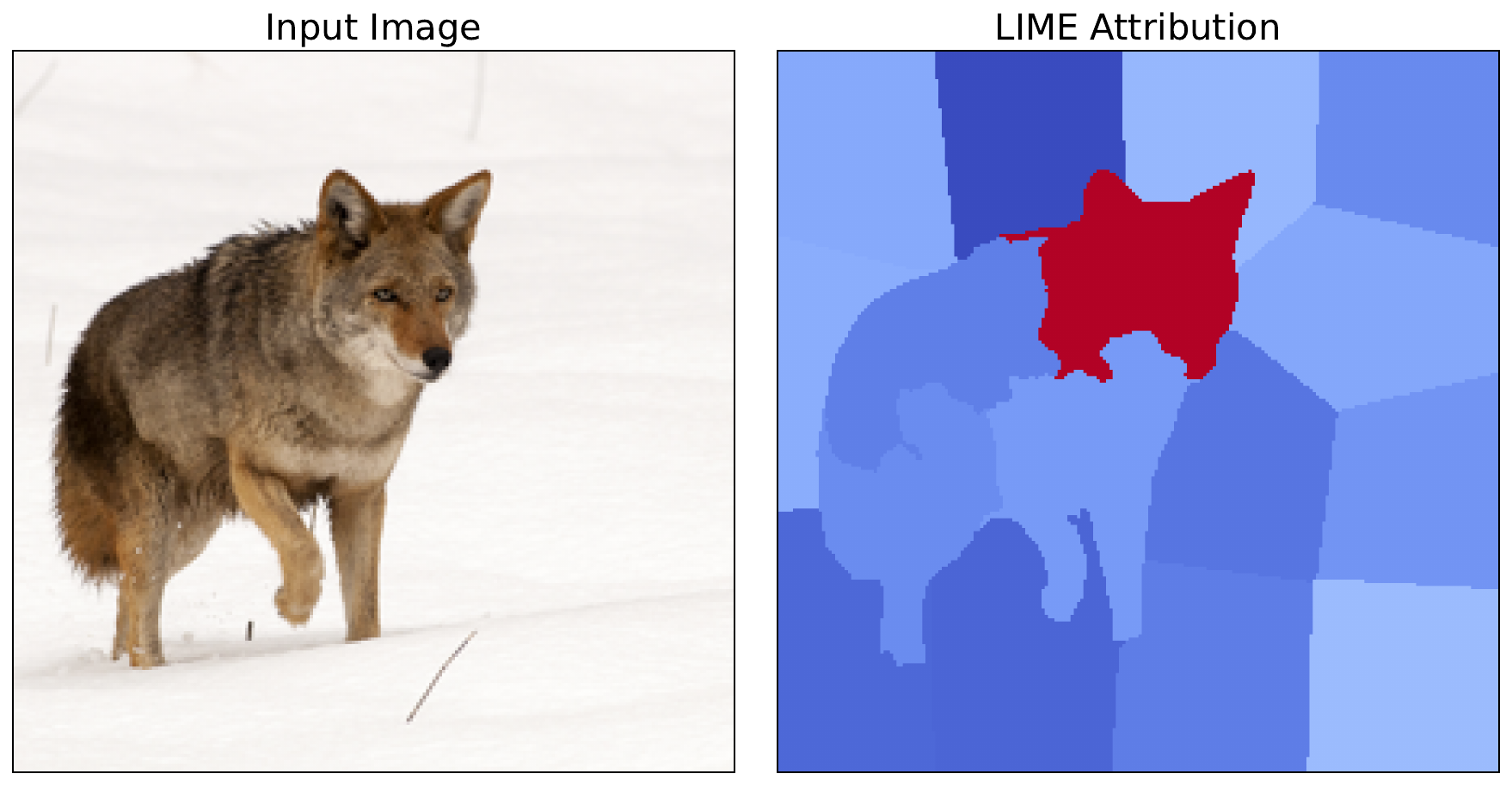

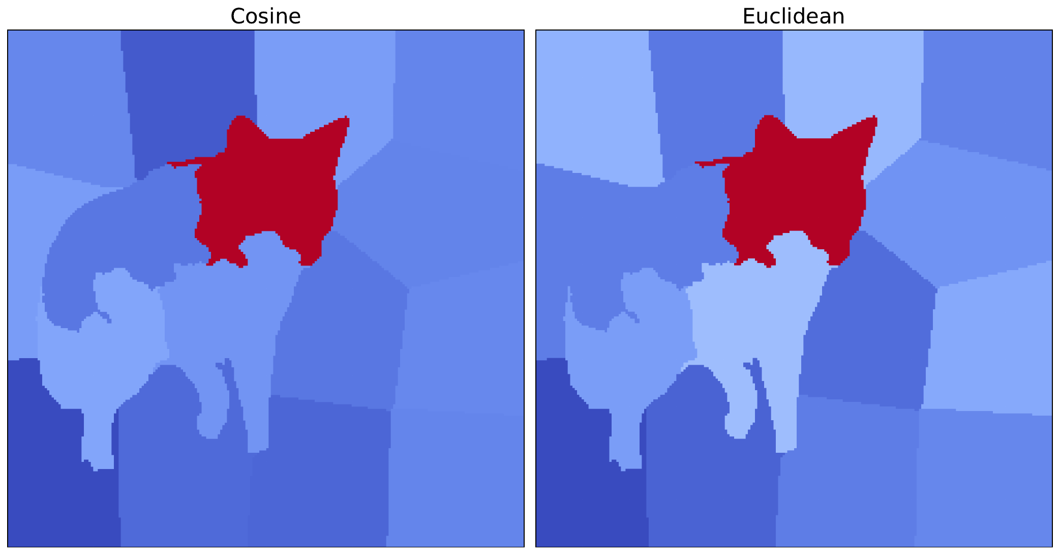
Euclidean distance metric

Up until now, we have used the default parameters from the Captum implementation of LIME. By default, this includes using the cosine distance metric to weight the individual samples. However, it is not immediately clear which metric is appropriate for a given problem. As mentioned, in the LIME paper, the researchers suggest using cosine for text problems and Euclidean for image problems [4]. So, it is worth explaining how you can implement Euclidean distance.

To do this, we will use the euclidean_similarity_func function below. During each iteration, the LIME attribution function will pass in the perturbed_interpretable_input (line 7). This is the binary vector, based on the feature_mask showing which superpixels have been perturbed (e.g., \([1,1,0,0,1,...]\)). We use this to create a vector of all ones with the same number of elements (lines 25-26). This is the same as the number of features/superpixels (line 25).

We find the distance between the two vectors using the Euclidean distance (line 29). We also need to calculate the kernel width. As mentioned in the theory section, the LIME paper recommends \(0.75 \times \sqrt{\text{number of features}}\) when working with the Euclidean distance (line 32). Finally, we obtain our weight by passing the distance and kernel_width into the Gaussian kernel (line 35).

from typing import Tuple, Union, Any
import torch.nn.functional as F

def euclidean_similarity_func(
    original_input: Union[torch.Tensor, Tuple[torch.Tensor, ...]],
    perturbed_input: Union[torch.Tensor, Tuple[torch.Tensor, ...]],
    perturbed_interpretable_input: torch.Tensor,
    **kwargs: Any
) -> torch.Tensor:
    """
    Calculate similarity weights using Euclidean distance.

    Args:
        original_input: Original input tensor
        perturbed_input: Perturbed input tensor
        perturbed_interpretable_input: Binary vector of interpretable features [1 x num_features]
        kernel_width: Width parameter for exponential kernel (sigma)
        **kwargs: Additional arguments (baselines, feature_mask, etc.)

    Returns:
        Weight (similarity) for this sample
    """

    # Create original binary vector (all superpixels on)
    num_features = perturbed_interpretable_input.shape[1]
    original_binary = torch.ones(1, num_features, device=perturbed_interpretable_input.device)

    # Calculate distance (Euclidean)
    distance = torch.norm(original_binary - perturbed_interpretable_input, p=2)

    # Calculate kernel width
    kernel_width = 0.75 * np.sqrt(num_features) # LIME paper default

    # Apply exponential kernel
    weight = torch.exp(-(distance ** 2) / (kernel_width ** 2))

    return weight

To implement LIME with this distance metric, the code is similar to before. The only difference is that we pass in this new distance function when initialising the LIME object (line 3). We also process and visualise the resulting attribution as before. You can see the result alongside the original cosine version in Figure 6.

# Get LIME attribution
lime = Lime(model, 
            similarity_func=euclidean_similarity_func)
attr = lime.attribute(
    img_tensor, 
    target=target_class, 
    feature_mask=feature_mask,
    n_samples=500)

We can see that the most important superpixel, containing the coyote's head, is the same for both distance metrics. As this is significantly more important in each case, the conclusions we can draw from both methods are similar. However, there are still some minor variations in the other superpixels. This shows how distance metrics can lead to different saliency maps and potentially different results for other images.

These approaches to weighting are an important concept for the next method we look at: KernelSHAP. This method is very similar to LIME with one key difference. That is, their weighting approach. With KernelSHAP, coalition-size-based weights from Shapley theory allow us to approximate Shapley values. The rest of the LIME framework we discussed here remains the same.

Challenge

Apply LIME using a different distance metric, such as the Hamming distance.

References

- Achanta, Radhakrishna, Shaji, Appu, Smith, Kevin, et al. (2012). SLIC superpixels compared to state-of-the-art superpixel methods. IEEE transactions on pattern analysis and machine intelligence, 34(11), 2274--2282.
- Felzenszwalb, Pedro F, Huttenlocher, Daniel P (2004). Efficient graph-based image segmentation. International journal of computer vision, 59, 167--181.
- Slack, Dylan, Hilgard, Sophie, Jia, Emily, et al. (2020). Fooling lime and shap: Adversarial attacks on post hoc explanation methods. Proceedings of the AAAI/ACM Conference on AI, Ethics, and Society, 180--186.
- Ribeiro, Marco Tulio, Singh, Sameer, Guestrin, Carlos (2016). Why should i trust you? Explaining the predictions of any classifier. Proceedings of the 22nd ACM SIGKDD international conference on knowledge discovery and data mining, 1135--1144.
Get the paid version of the course. This will give you access to the course eBook, certificate and all the videos ad free.