Deep learning models rely on certain features in an image to make decisions. These are aspects like the colour of a stop sign, the texture of a cat’s fur or the outline of someone’s face. While occlusion saliency maps cannot give these detailed explanations, they can tell us the locations of features. That is, which pixels a model is using to make a prediction.
Occlusion is a permutation-based method for explaining machine learning models. It works by systematically permuting (or masking) regions of an input image. We can understand the importance of a given region by comparing the model’s output to the output using the original, unpermuted image. When we combine the results for all regions, we can generate an occlusion-based saliency map.
Specifically, we are going to:
- Explain the theory behind occlusion-based methods
- Discuss the limitations of the method
- Demonstrate their application using the Captum Python package
In the end, we will see that occlusion is a simple yet effective technique for interpreting model predictions. However, this simplicity leads to one of its biggest weaknesses — omitting global context.
The theory behind occlusion-based saliency maps
What is occlusion?
Occlusion is a type of permutation-based interpretability method where specific regions of an input image are masked or replaced with a neutral value (e.g., black, zero, or the mean pixel intensity) [2]. This mask is referred to as an occlusion patch or window. By observing the change in a model’s prediction when different parts of the image are occluded, we can see which spatial regions contribute most to the decision-making process.
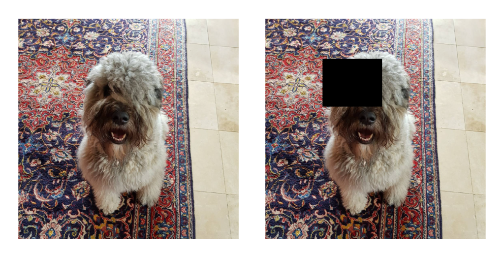
Take Figure 1 for example. We have occluded the image of a dog with a black occlusion patch. Suppose we feed both these images into a model to get a predicted probability for the dog class. The prediction on the original image is referred to as the baseline. If the probability corresponding to the occluded image decreases significantly compared to the baseline, we can say the occluded region is important for the prediction.
How occlusion is used to create saliency maps
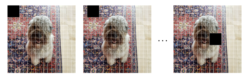
To create a saliency map with occlusion, we repeat this process systematically with the same occlusion patch. The patch moves across the image in a sliding window fashion by a given number of pixels (or stride). For example, in Figure 2, suppose the grid shows individual pixels. We have a black occlusion patch with dimension (3,3) moving with a stride of 1.
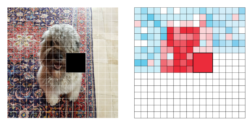
For each step, we compare the occluded prediction to the baseline prediction. The difference is referred to as an importance score. We add this to the pixels in the saliency map at the same location as the occlusion patch in the image. Looking at Figure 3, the same value is added to all 9 pixels in the saliency map. Here, the red squares indicate a higher importance score. However, keep in mind that both large negative and positive values indicate important regions.
The final step is to normalise the saliency map. The scores will be biased as some pixels will be occluded more than others. So we divide each pixel’s accumulated importance by the number of times it was occluded. This allows us to interpret the saliency maps in terms of the unit of the prediction. For example, a probability or a continuous value. We can further normalise the values between 0 and 1 to interpret the map in terms of the percentage of maximum saliency.
This general process is always the same, but we do have a few choices to make:
- Occlusion patch size – This includes the width, height and whether to occlude all channels simultaneously or individually.
- Occlusion patch value – You can use a colour like grey or black. You can also use the mean or random value from an image.
- Stride – the number of pixels the occlusion patch moves by.
These choices provide some flexibility over the method. However, as we will see in the next section, they lead to a limitation.
The limitations of occlusion
While occlusion-based saliency maps are simple and effective, they come with several limitations that must be considered when interpreting results.
The saliency map depends on your choices
The quality and interpretability of the saliency map are heavily influenced by the choices made during occlusion [1]. Different patch sizes, occlusion values and strides can lead to significantly different results. We will see this when we apply the method in the next section. Ultimately, there is no universally optimal set of parameters. This makes the method less objective compared to other interpretability methods.
It is computationally expensive
Occlusion requires multiple forward passes through the model. If the stride is too small, the occlusion patch moves in small increments, meaning hundreds or thousands of predictions might be required to generate a saliency map. For large images or deep neural networks, this method can take a long time to compute, making it impractical for real-time applications or large-scale datasets.
It does not take into account global context
A model may rely on complex relationships between distant regions, but occlusion treats each region independently. That is, we only mask one region at a time. Ultimately, this means we cannot capture the full context of how different parts of an image interact. Take Figure 4 for example. The model would likely produce a high probability for a dog prediction. To significantly decrease the probability, we may have to occlude all three of their face simultaneously.
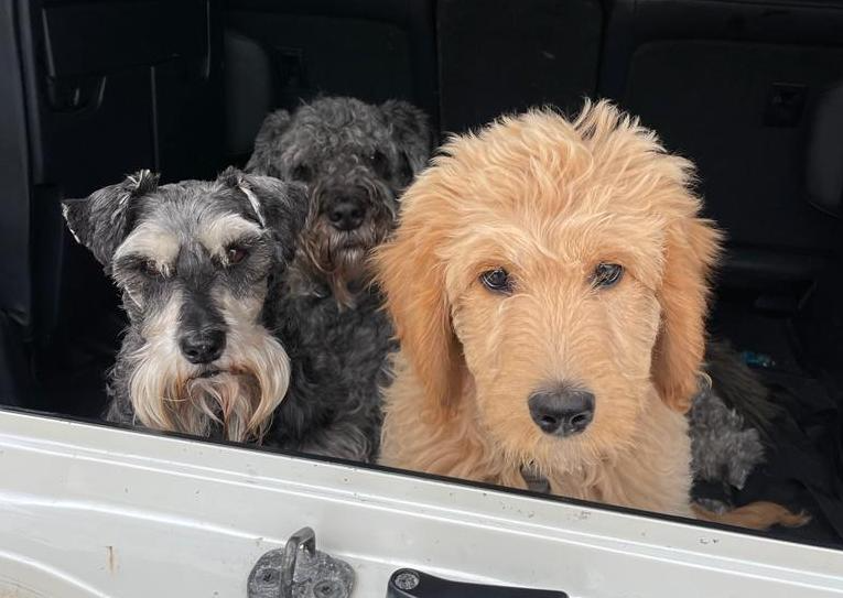
This limitation is where SHAP comes in. It is another permutation method that will occlude all combinations of regions in an image. Regions that interact or are only important when combined will now be highlighted. The problem with this approach is an even higher computational cost. So, although occlusion has its limitations, it can still provide a simple and useful method for interpreting models.
Applying Occlusion Saliency Maps with Captum and Python
We start with our imports. We will be using the Occlusion module from the Captum package (line 10). We will load our model from Hugging Face (line 8). In the src directory, there is a folder called modelling. We navigate to this folder (line 14), load the CNN class from network.py (line 16) and the ImageDataset class from datasets.py (line 17). These are the same classes used to train the model.
import torch
import numpy as np
import matplotlib.pyplot as plt

import glob
import cv2

from huggingface_hub import hf_hub_download

from captum.attr import Occlusion

# Change sys path to import from parent directory
import sys
sys.path.append('../modelling')

from network import CNN
from datasets import ImageDataset
Load model and dataset
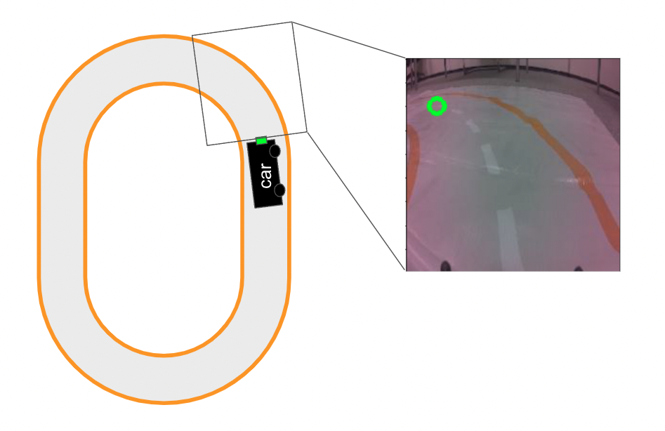
We will be working with a model trained on the road following dataset. As seen in Figure 5, this dataset is used to train a model that directs an automated car. There is a camera on the front of the car and a model uses the images to make predictions. The predictions are then used to direct the car.
We load a CNN trained on this dataset (lines 2-7). We also move this model to a GPU (lines 10-13) and set it to evaluation mode (line 14). Specifically, we are loading the model trained on images collected in a single room (line 3). In the lesson on aggregating saliency maps, we will explore how using images from multiple locations can reduce bias in this model.
# Download the model from Hugging Face Hub
model_path = hf_hub_download(repo_id="a-data-odyssey/XAI-for-CV-models",
                             filename="models/car_single_room/model.pth")

# Load the model
model = CNN(num_classes=1,input_dim=224)
model.load_state_dict(torch.load(model_path))

# Set the model to evaluation mode
device = torch.device('mps' if torch.backends.mps.is_built()
                      else 'cuda' if torch.cuda.is_available()
                      else 'cpu')
model.to(device)
model.eval()
We load the validation dataset from the single room version of the dataset (lines 1-6). You can find this on Kaggle. Setting num_classes = 1 will create an ImageDataset object for a regression model (line 5). Let’s take a closer look at one of the instances.
base_path = "../../data/auto_car/single_room"
val_paths = glob.glob(base_path + "/val/*.jpg")
# Load the validation data
val_data = ImageDataset(val_paths,num_classes=1)
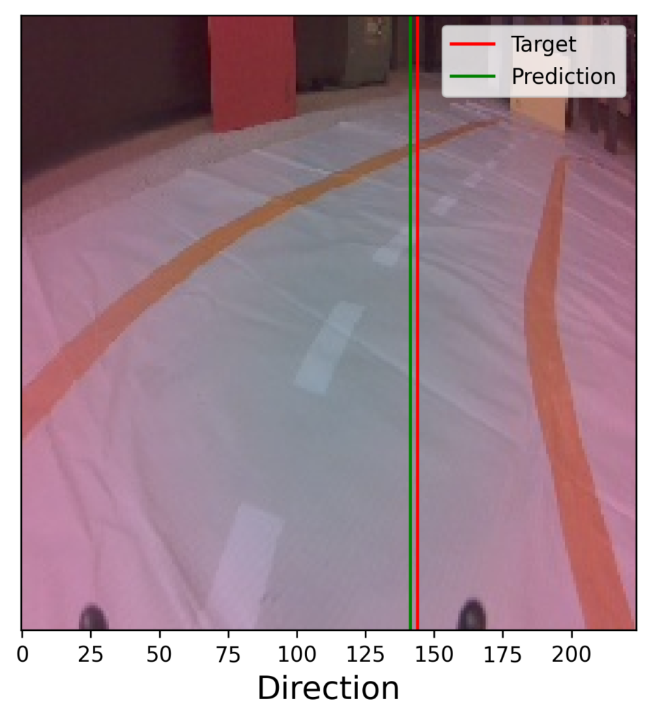
print(f"Validation data: {val_data.__len__()}") #300We load an example image (line 1), move it to the GPU (line 2) and add a batch dimension (line 3). We then use our CNN to get the direction prediction from this image (line 6). We format the prediction, target and example image (lines 9-13) and display them (lines 16-24). You can see the results in Figure 6.
image, target = val_data.__getitem__(1)
image = image.to(device)
image = image.unsqueeze(0) # Add batch dimension

# Get prediction
pred = model(image)

# Format prediction, target and image
pred = pred.item()
target = target.item()
display_image = image.cpu().detach().squeeze(0).permute(1,2,0).numpy()
display_image =display_image*255
display_image = display_image.astype(np.uint8)

# Plot image
plt.imshow(display_image)
plt.axvline(x=target, color='r',label='Target')
plt.axvline(x=pred, color='g',label='Prediction')
plt.legend()

# Label axis
plt.xlabel('Direction',size=15)
plt.yticks([])
You can see the image taken by the automated car and the target direction. The direction is given by coordinates on the x-axis. Lower values (less than 122) indicate the car should turn left, and higher values (greater than 122) indicate the car should turn right. In this case, the car should make a gradual right turn. Thankfully, the predicted direction is not too far off. Let’s see how we can use occlusion to understand how the model is making this prediction.
Occlusion-based saliency maps
We start by creating an occlusion object for our model (line 2). We then use the object’s attribution function to create an occlusion saliency map for our example image (lines 5-7). Consider the following parameters:
- sliding_window_shapes gives the size of the occlusion patch. We have a patch of size 32 by 32 pixels. Using 3 as the first dimension means we will apply the patch to all channels simultaneously.
- strides will move the patch 16 pixels at a time.
- By default, an occlusion value of 0 is used. Later, we will change this with the baselines parameter. This is not the same as the baseline prediction we discussed above.
# Define the occlusion object
occlusion = Occlusion(model)

# Apply occlusion
attributions = occlusion.attribute(image,
                                   strides=16,
                                   sliding_window_shapes=(3, 32, 32))
We format the attributions as a numpy array (line 2). This has a shape of (3, 244, 244), which are the same dimensions as the example image. There is a saliency map for each of the channels. However, because of the sliding_window_shapes parameter, every saliency map will be the same. So we select the first one (line 6). We can now display this map.
# Convert to numpy and plot the saliency map
saliency_map = attributions.squeeze().cpu().detach().numpy()
print(saliency_map.shape) # (3, 224, 224)
# Select one channel as they are all the same
saliency_map = saliency_map[0]
print("Min:", saliency_map.min()) # -53.7
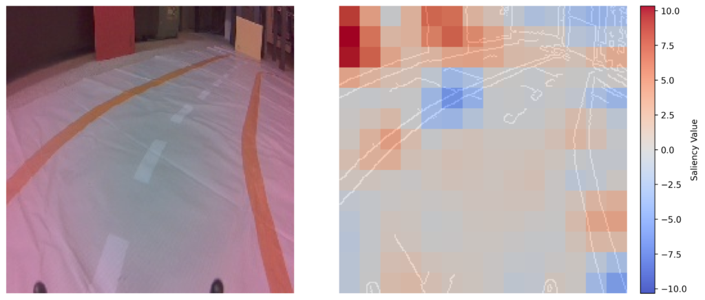
print("Max:", saliency_map.max()) # 44.3For clarity, we will plot the saliency map on top of an edge version of the input. This is created using Canny edge detection (lines 2-3). We then plot the example image, target and prediction (lines 8-14) alongside our saliency map (lines 17-33). We add a colour bar (lines 32-33) and make sure this is centred on 0. This is done by taking the maximum of the absolute saliency (line 22) and using it to set symmetrical bounds (lines 28-29). You can see the results in Figure 7.
# Create edge image
grey_image = cv2.cvtColor(display_image, cv2.COLOR_RGB2GRAY)
edge_image = cv2.Canny(grey_image, 50, 100)
fig, ax = plt.subplots(1, 2, figsize=(12, 5))
# Display image and prediction
ax[0].imshow(display_image)
ax[0].axvline(x=target, color='r',label='Target')
ax[0].axvline(x=pred, color='g',label='Prediction')
ax[0].legend()
ax[0].set_yticks([])
ax[0].set_xlabel('Direction',size=15)
# Display saliency map
ax[1].imshow(edge_image , cmap='gray')
ax[1].set_xticks([])
ax[1].set_yticks([])
# Normalize saliency map values
abs_max = np.max(np.abs(saliency_map))
# Overlay saliency map with color bar
saliency_plot = ax[1].imshow(saliency_map,
alpha=0.9,
cmap='coolwarm',
vmin=-abs_max,
vmax=abs_max)
# Create colorbar
cbar = fig.colorbar(saliency_plot, ax=ax[1], fraction=0.046, pad=0.04)
cbar.set_label("Saliency Value")The result of all that work is a saliency map that can be interpreted in terms of the unit of the target variable. Looking at Figure 7, white locations did not play an important role in the prediction. In other words, they did not have a significant influence on the car’s direction. For the red squares, when we masked out these areas, the prediction was lower than the baseline prediction. This led to a higher importance score. In other words, these areas cause the car to turn right. Similarly, the blue areas cause the car to turn left.
Overall, there is more red than blue, which aligns with the overall direction of the car. However, keep in mind that, unlike SHAP, occlusion does not have the efficiency property. This means that if you add up all the individual saliency values, they will not give you the original prediction. In other words, these show how much the prediction would change if you masked the square, but not how much that collection of pixels has contributed to the prediction.
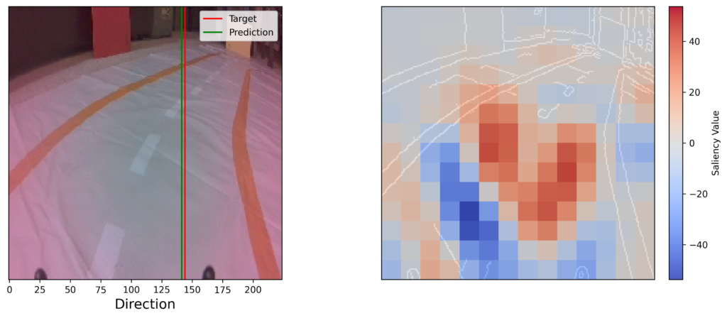
Regardless of the precise interpretation, the saliency map provides some valuable insight into the model. A key takeaway is that the most important pixels appear to be on the track. This is good news as we would expect a robust model not to use background pixels. However, there are still a few background pixels that do not have a saliency of 0. We explore this idea further in a later lesson when we try to improve the model by training on images from multiple rooms.
Alternatives to the default occlusion saliency map
For now, we will explore some alternatives to the saliency map above. This includes scaling the map, creating individual maps from each channel and using a different occlusion value.
Scaling between 0 and 1
In some cases, it may make more sense to give the saliency in terms of a percentage of maximum saliency. This is particularly true when working with logits or probabilities from classification problems. To do this, we take the absolute value of the saliency map and divide by its maximum value (line 2). We calculated this previously. We then visualise the saliency map just as before.
# Percentage of occlusion
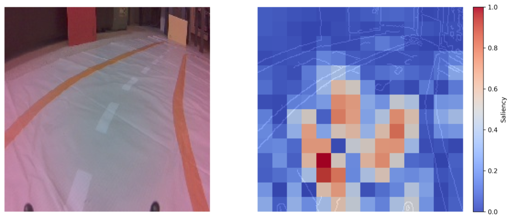
per_saliency_map = np.abs(saliency_map) / abs_maxYou can see the output in Figure 8. We now only have values between 0 and 1. Using this map, it is clearer that the center of the track is the most important region for the prediction. This is because both high positive and negative values will have a large percentage. The downside is that we do not know the direction in which the regions have changed the predictions.
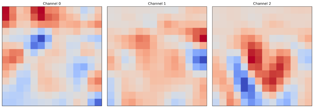
Saliency map for individual channels
Another alternative is to produce saliency maps for individual channels. To do this, we need to adjust the strides (line 3) and patch size (line 4) so that the value for their first dimension is one. When we visualise each saliency map (lines 6-13), you can see they are all different.
# Calculate for individual channels
attributions = occlusion.attribute(image,
                                   strides=(1, 16, 16),
                                   sliding_window_shapes=(1, 32, 32))

saliency_map = attributions.squeeze().cpu().detach().numpy()

fig, ax = plt.subplots(1, 3, figsize=(15, 5))
for i in range(3):
    ax[i].imshow(saliency_map[i], cmap='coolwarm')
    ax[i].set_title(f"Channel {i}")
    ax[i].set_xticks([])
    ax[i].set_yticks([])
Looking at the output in Figure 8, this approach typically doesn’t produce much insight for standard image problems. It may be able to tell you if one channel is more important than another. You may find more benefit when dealing with multispectral images. Like in the previous lesson on Permutation Feature Importance.
Mean intensity occlusion value
The final adjustment is the most important. As mentioned, the parameters of the occlusion process can impact its output. This includes the stride, size of the occlusion patch and value of the occlusion patch. To see this, we will use the mean value for each channel as the occlusion value (line 2). We then use this to set the baseline parameter (line 9). This will set the new value for the occlusion patch. Previously, this parameter was given the default value of 0. We can then visualise the map as before.
# Get mean of each channel
mean_baseline = torch.mean(image, dim=(2, 3), keepdim=True)
print(mean_baseline)

# Apply Occlusion
attributions = occlusion.attribute(image,
                                   strides=16,
                                   sliding_window_shapes=(3, 32, 32),
                                   baselines=mean_baseline)
Looking at the output in Figure 9, you can see the saliency map is quite different to before. Now it appears as though the background pixels are the most significant to the model’s prediction. This is a worrying result as we would expect the model to only use pixels of the track. Otherwise, if we move to a new room, the car might struggle to make correct turns.
When understanding these results, you need to consider how the occlusion value can introduce bias. The mean value may be skewed. You can see that the majority of the image is taken up by the track. So, the resulting mean may be close to the values of the track. In other words, we may end up with a grey-ish occlusion square.
When we occlude the background pixels with this value, they change a lot. This leads to a large change in the prediction. In comparison, when we occlude the track pixels, they do not change as much. As further evidence, note that the orange bars have become significant. This may be because they are different to the mode colour of the track. A similar bias may be introduced using the default value of 0. Ultimately, the problem is that saliency scores will depend on how different the pixels are from the occlusion value.
One way to get around this is to choose a random value for each channel from the image. We can use that as the occlusion value and repeat the same process as above. In this case, you will need to repeat the process at least 3 times and take an average. This will reduce the variability and bias of any given random occlusion value.
Challenge
This leads us to the challenge: create an occlusion-based saliency map using random occlusion values. Do the results align with the default or mean occlusion value?
I hope you enjoyed this article! See the course page for more XAI courses. You can also find me on Bluesky | Threads | YouTube | Medium
Additional Resources
Datasets
Conor O’Sullivan (2024). Road Following Dataset. (CC BY 4.0) https://www.kaggle.com/datasets/conorsully1/road-following-car
References
[1] Rokas Gipiškis and Olga Kurasova. Occlusion-based approach for interpretable semantic segmentation. In 2023 18th Iberian Conference on Information Systems and Technologies (CISTI), pages 1–6. IEEE, 2023.
[2] MD Zeiler. Visualizing and understanding convolutional networks. In European conference on computer vision/arXiv, volume 1311, 2014.
Get the paid version of the course. This will give you access to the course eBook, certificate and all the videos ad free.