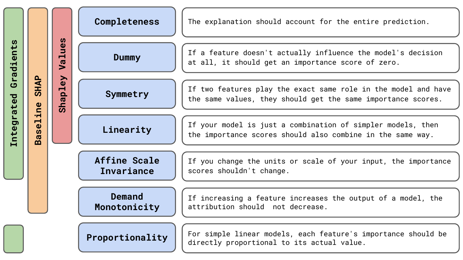
Axioms are desirable mathematical properties of XAI methods. As we discuss the 7 common axioms in Figure 1, you will see they all have an intuitive justification for why we would expect a good explanation to satisfy them. We will also touch on which methods satisfy certain axioms and how you can use this information to choose the best XAI method for your problem.
Before you get stuck into the article, here is the video version of the lesson.
We ended the lesson on Taxonomy with the axiom grouping. That is, we can classify XAI methods as either being based on a heuristic or one that is derived from or satisfies certain axioms. It may seem obvious that we would want to use the latter methods. However, axioms often come with the cost of increased complexity and computational time. Whether that trade-off makes sense depends on what you want to use XAI for. So, before we get into the technical details, let's understand...
Should you worry about axioms?
A key consideration is that satisfying axioms often comes with additional complexity and computation cost. Methods like Integrated Gradients (IG) and Shapley Values satisfy many axioms. Yet, IG can take up to 50 backwards passes to converge, and methods for approximating Shapley Values are even more computationally expensive. Faster, heuristic-based methods can speed up the iterative process of model development. The inherent simplicity of these methods can also make them easier to explain to colleagues.
If you are reading this from industry (sorry), these properties of heuristic-based methods are likely appealing. Odds are you are using XAI to debug a model. Speed and simplicity will make this process easier. This is especially true if you are trying to debug large models or using many images. XAI is also only one of the tools, along with data exploration, evaluation metrics and domain knowledge, at your disposal. To be effective, XAI needs to be reliable and, to a certain extent, faithful, but it does not necessarily have to satisfy strict mathematical requirements.
On the other hand, axioms can help ensure that an XAI method is reliable — behaves consistently and sensibly in practice. Less directly, they can ensure a method is faithful — it reflects the model’s true decision-making process. Yet, as we discuss in the lesson on Evaluation, there are other ways to evaluate for these properties empirically. Many of these are more intuitive than mathematical proof for various axioms. In general, if you are concerned with practicality, then axioms are not the most useful thing to focus on.
If from academia (even more sorry), then you may be more concerned with axioms. They provide a useful mathematical lens for understanding XAI methods, and you generally won't be as concerned with development time. Additionally, a large part of XAI research is aimed at developing explanations for model predictions in a way that humans can understand. This is a higher burden than debugging a model, and reliability and faithfulness are more important. Axioms can help ensure that an explanation has these properties or help us develop new methods that do have them.
We should also keep in mind that there is no method that can satisfy all desirable axioms. This leads to limitations from an axiomatic point of view and differences in resulting saliency maps. In general, it is good practice to use multiple methods to mitigate shortcomings of any individual method. When debugging a model, you may be able to use multiple heuristics like Grad-CAM, Guided Backpropagation or simple axiom-based methods like DeepLIFT to make up for the lack of axioms.
Seven common axioms
Technically, axioms are foundational statements used to derive mathematical objects like XAI methods. Here, we refer to axioms as all the mathematical properties that a method satisfies but is not necessarily derived from. The research in this area can be quite confusing. Different properties are referred to with different names. Also, as the field has progressed, initial proofs have been disproven, or methods have been shown to satisfy different axioms. So let's summarise some of the most important ones.
Completeness
Completeness means that the sum of all feature attributions equals the difference between the model’s prediction for the input and a baseline/reference prediction [1, 2]. This axiom ensures the explanation accounts for the entire prediction. For image data, it means that if we add up the attribution for each individual pixel \(A_i\) we would get the difference between the predicted score when using the original input (\(X\)) and a baseline (\(X^0\)):
\[
\sum_{i=1} A_i = f(X) - f(X^0)
\]
This property is also referred to as efficiency [3], local accuracy [4] or the summation-to-delta property [5]. There will also be differences in what is used as a baseline. For example, with SHAP, we use the expected prediction over a sample of images, \(E[f(X)]\). In this case, completeness means we attribute the entire difference between a prediction and the average prediction.
This property is particularly important to DeepLIFT [5]. This method was designed as a set of rules to calculate \(C_{\Delta x_i\Delta y}\). This is the contribution of change in an input value, \(\Delta x_i\), to change in the output \(\Delta y\) when comparing the values using the original input (\(X\)) and a baseline (\(X^0\)). The rules propagate these contributions through the network so that at every layer, the summation-to-delta property, \( \sum_i C_{\Delta x_i\Delta y} = \Delta y \), is satisfied. Although this approach does not necessarily mean the axiom will always be satisfied.
It has been shown that DeepLIFT can violate the completeness axiom for more complex methods. Specifically, for networks with multiplicative interactions like RNNs [6]. So, although DeepLIFT could be thought of as an axiomatic approach, it is closer to a heuristic. In comparison, another gradient-based method called Integrated Gradients does satisfy completeness, as well as KernelSHAP under certain conditions [3].
Dummy
A dummy feature is one that does not affect the prediction. The dummy property is that these features should get zero attribution [3, 2]. This axiom is also referred to as Sensitivity(b) [1] and missingness [4]. Formally, we can say that feature \(i\) is dummy if for a function \(f\) and any two values \(x_i\) and \(x'_i\) and other features \(x_{N\setminus i}\) then:
\[
f(x_i; x_{N\setminus i}) = f(x'_i; x_{N\setminus i})
\]
In other words, we always get the same prediction regardless of the feature's value. These must be given zero attribution, as it prevents irrelevant features from being highlighted. For computer vision, feature \(i\) can be an individual pixel or a cluster of pixels. For dummy features, the corresponding pixels in the saliency will be grey/black, depending on the background colour.
Symmetry
Two features are symmetric if swapping them in the function does not change the output. That is, we have:
\[
f(x, y) = f(y, x)
\]
for all values of x and y. The symmetry axiom is that if these features have the same values, \(x=y\), then they should be given the same attribution. For example, a fraud model may treat transaction amounts from merchants A and B identically. Swapping these should not change the fraud probability, and they should be given equal attribution if the transaction values are the same.
In practice, perfect symmetry in input features is rare. This is particularly true for computer vision. However, for an illustrative example, suppose we have an image classifier used for facial recognition. This architecture processes the left and right eye regions using identical convolutional filters. As a result, the function treats the two pupils symmetrically. Swapping the intensity of the left-eye pupil pixel and the right-eye pupil pixel does not change the model output. If in a particular input image those pixels have the same value, then the Symmetry axiom requires that their attributions must also be equal.
Linearity
Suppose a model \(f\) is a linear combination of two other models \((a f_1 + b f_2 )\). The linearity axiom requires the attributions for \(f\) to be the weighted sum of the attributions for \(f_1\) and \(f_2\) with weights \(a\) and \(b\) respectively [3, 1, 2]. For example, for a random forest, the attribute of a feature should be its mean attribution across all the individual decision trees. Similarly, if we sum the outputs of two neural networks, then we can find the overall attribution using the attributions from the individual networks. That is, if they have the same input and output.
These last four axioms, Completeness, Dummy, Symmetry and Linearity were used to derive the Shapley values [7]. This is an influential formula for cost-sharing in game theory which has been adapted to machine learning [4, 8, 9]. However, we must keep in mind that the original formula applies to discrete teams/coalitions in a game. The many adaptations or approximations of this do not necessarily have these properties.
For example, KernelSHAP is the most popular approximation [4]. This approximation assumes feature independence, and it has been shown that if this assumption is violated, then both the dummy and linearity axioms may fail [3]. As we will see in the lesson on KernelSHAP, this is particularly concerning for image data. The structure of images means that pixels and groups of pixels are highly likely to be dependent. This means that when applying KernelSHAP to image data, the output may be unreliable.
The next three may seem niche, but they are useful in comparing two methods: baseline SHAP (BShap) [3] and IG [1]. Both methods satisfy 6 of the 7 axioms we discuss here, with a different axiom not satisfied. However, as we will see, BShap is not appropriate for image problems, leading us to conclude that IG is the most sound option from an axiomatic point of view.
Affine Scale Invariance
An affine transformation is a geometric transformation that maintains:
- all points on a line stay on the line (collinearity)
- ratios of distances between points on a line
They include combinations of operations like shearing, rotation, translation, and scaling. For example, using the latter two operations, we can scale a feature using min-max scaling:
\(x' = \frac{x-min(x)}{max(x)-min(x)}\)
Affine scale invariance is when an attribution of a feature does not change after an affine transformation has been applied. That is, provided the functions using the original and transformed features give the same predictions [3, 2]. This means, for tabular data, it would not matter if a feature was encoded using kilometers vs meters or Celsius vs Fahrenheit. For image data, we should get the same saliency maps regardless of whether we scale pixels by dividing by 255 or not. Intuitively, this makes sense as we are using the same information but on a different scale.
Demand Monotonicity
A function is monotone in a feature if it does not decrease when we increase the feature (or vice versa). Demand monotonicity means that if we increase the values of such a feature, then the feature's attribution should not decrease [3]. Suppose we develop a model to classify cloudy images. A monotone feature constructed at deep levels of the network could be the number of white pixels in an image. So, if we have two images, one with more white cloud pixels, the attribution for this feature should be at least as large as the attribution in the image with fewer cloud pixels.
Proportionality
If a model's output can be expressed as a function of the sum of all features:
\[
f(x) = g ( \sum x )
\]
Then the proportionality axiom [3, 2] requires that the attribution assigned to a feature must be proportional to its value:
\[
A_i = c x_i
\]
By definition, linear models can always be expressed as a sum of features. Intuitively, we want an attribution to be proportional to a feature's value. More specifically, the attribution should be the feature value times its weight in the linear equation. This also makes sense for non-linear models that have collapsed into a linear one. For example, we could use a CNN to count the number of edge pixels in a binary image. Despite having the capacity to model more complex relationships, the CNN may simply sum the values in the input to get an accurate prediction. In this case, all edge pixels should be given the same attribution.
Choosing XAI methods based on axioms
As mentioned, these last three axioms are important as they help us compare two methods: BShap [3] and IG [1]. BShap satisfies all common axioms except proportionality, and IG satisfies all except demand monotonicity [3]. Between these two, it may seem like demand monotonicity is the stronger axiom. However, when it comes to computer vision, IG may still be the best method from an axiomatic point of view.
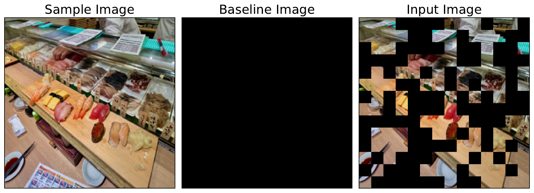
This is because of the way BShap uses a baseline image. As we will see in the lesson on IG, the method looks at many images on a straight line path from a baseline to the input image. In comparison, BSHAP uses different combinations of pixels in the baseline and sample image. For example, as seen in Figure 2, if we use a black image as a baseline, then random parts of the input image will be black. This can lead to problems as these constructed input images are unrealistic and likely the model has not seen similar ones in the training data.
Still, we stress that axioms are an active area of research. A consensus is still being formed. For example, some of the initial properties stated by IG [1] were disproved [10, 11]. Later work provided the above result [3], which has since been expanded on [2]. However, what remains true is that no method can satisfy all desirable axioms. Combined with the problems we discussed in the lesson on Evaluation, it leads to the first limitation we will discuss in the next lesson.
Which leads us to the...
Challenge
Try to find some other axioms not mentioned in this lesson.
I hope you enjoyed this article! See the course page for more XAI courses. You can also find me on Bluesky | YouTube | Medium
Additional Resources
- YouTube Playlist: XAI for Tabular Data
- YouTube Playlist: SHAP with Python
Datasets
Conor O’Sullivan, & Soumyabrata Dev. (2024). The Landsat Irish Coastal Segmentation (LICS) Dataset. (CC BY 4.0) https://doi.org/10.5281/zenodo.13742222
Conor O’Sullivan (2024). Pot Plant Dataset. (CC BY 4.0) https://www.kaggle.com/datasets/conorsully1/pot-plants
Conor O'Sullivan (2024). Road Following Car. (CC BY 4.0). https://www.kaggle.com/datasets/conorsully1/road-following-car
References
- Sundararajan, Mukund, Taly, Ankur, Yan, Qiqi (2017). Axiomatic attribution for deep networks. International conference on machine learning, 3319--3328.
- Lundstrom, Daniel, Razaviyayn, Meisam (2025). Four axiomatic characterizations of the integrated gradients attribution method. Journal of Machine Learning Research, 26(177), 1--31.
- Sundararajan, Mukund, Najmi, Amir (2020). The many Shapley values for model explanation. International conference on machine learning, 9269--9278.
- Lundberg, Scott M, Lee, Su-In (2017). A unified approach to interpreting model predictions. Advances in neural information processing systems, 30.
- Shrikumar, Avanti, Greenside, Peyton, Kundaje, Anshul (2017). Learning important features through propagating activation differences. International conference on machine learning, 3145--3153.
- Ancona, Marco, Ceolini, Enea, \"Oztireli, Cengiz, et al. (2017). Towards better understanding of gradient-based attribution methods for deep neural networks. arXiv preprint arXiv:1711.06104.
- Shapley, Lloyd S, others (1953). A value for n-person games. Princeton University Press Princeton.
- (2014). Explaining prediction models and individual predictions with feature contributions. Knowledge and information systems, 41(3), 647--665.
- Chen, Hugh, Covert, Ian C, Lundberg, Scott M, et al. (2023). Algorithms to estimate Shapley value feature attributions. Nature Machine Intelligence, 5(6), 590--601.
- Lundstrom, Daniel D, Huang, Tianjian, Razaviyayn, Meisam (2022). A rigorous study of integrated gradients method and extensions to internal neuron attributions. International Conference on Machine Learning, 14485--14508.
- Lerma, Miguel, Lucas, Mirtha (2021). Symmetry-preserving paths in integrated gradients. arXiv preprint arXiv:2103.13533.
Get the paid version of the course. This will give you access to the course eBook, certificate and all the videos ad free.