
When it comes to saliency maps, Integrated Gradients (IG) is a strong, well-justified choice with solid theoretical foundations. It could even be considered the best gradient-based method from an axiomatic point of view. On top of this, it has an intuitive interpretation which helps when it comes to analyzing its explanations.
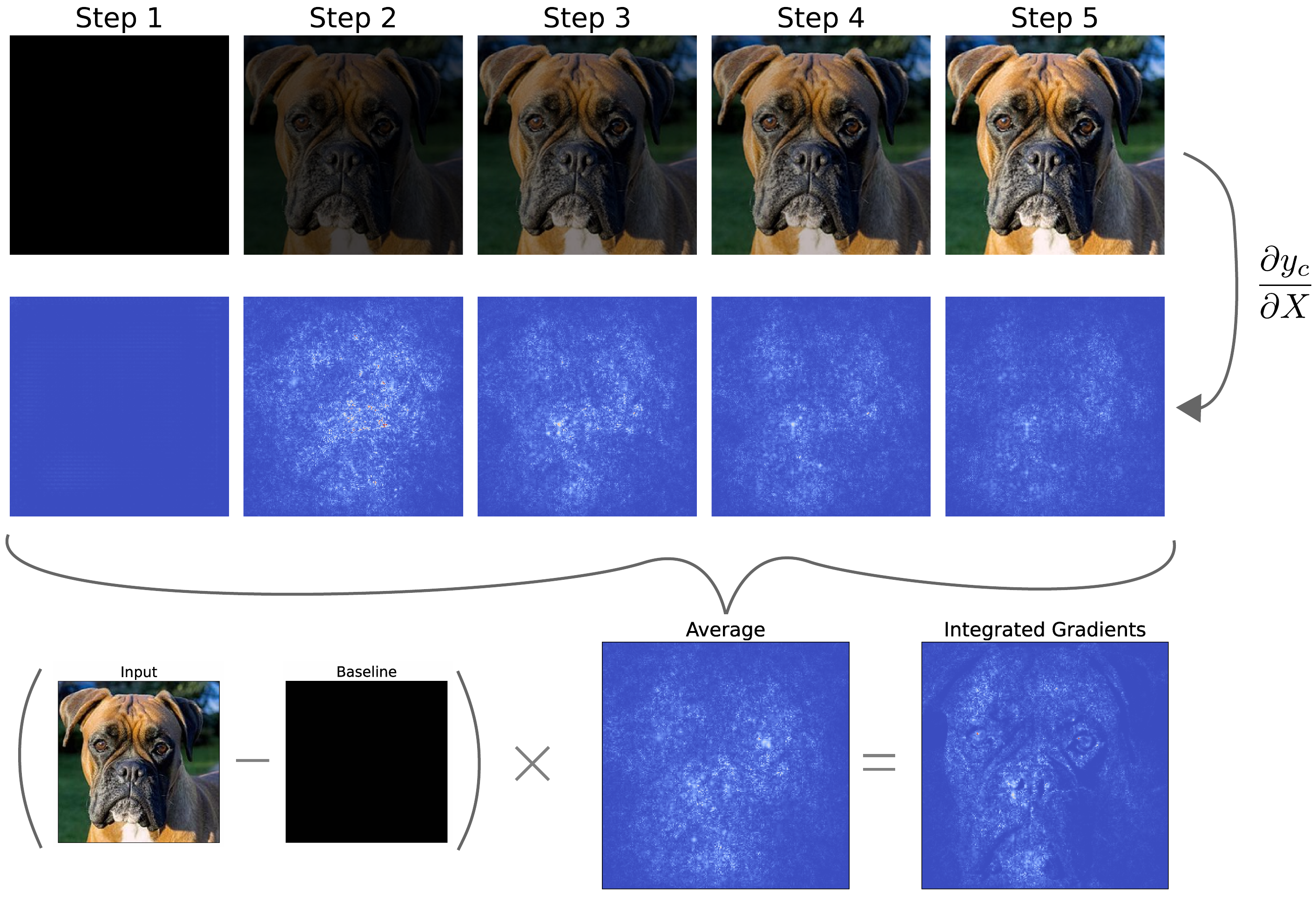
These benefits come from the way in which IG uses a baseline image. As seen in Figure 1, this is done by calculating the gradients for interpolated images along a path from the baseline to the original input image. Taking the average of all those gradients and multiplying by the difference between input and baseline gives us our final saliency map.
We will discuss the process behind IG in more depth. This will involve understanding the mathematics behind the method. We will also compare to how DeepLIFT uses a baseline, discuss the axioms IG satisfies and explain how to interpret the resulting saliency maps. To end, we will apply the method using Captum.
Before you get stuck into the article, here is the video version of the lesson.
The theory behind Integrated Gradients
To start, we calculate a straight line path from a baseline image, \(X^0\), to the original image, \(X\). Each step along the path will give us a new interpolated image. If we have \(m\) steps, then the interpolated image \(k\) is given by:
\[
X^0 + \frac{k}{m}(X - X^0)
\]
We saw the result of this in Figure 1. The first will be the baseline (e.g. black image), and with each step, we slowly reduce its contribution to the interpolated image until we get our original input image.
For each of the \(m\) steps, we feed the interpolated image into the model. We then calculate gradients w.r.t. the target logit, \(y^c\), using backpropagation. This is the same process used to find Vanilla Gradients, applied to different input images:
\[
\frac{\partial y_c}{\partial X} = \frac{\partial F( X^0 + \frac{k}{m}(X - X^0))}{\partial X}
\]
We then take the average gradient over all \(m\) steps:
\[
\frac{1}{m}\sum^m_{k=1} \frac{\partial F( X^0 + \frac{k}{m}(X - X^0))}{\partial X}
\]
The final saliency map is calculated by taking this average and multiplying it by the difference between the baseline and the original input image:
\[
IG(X) = (X-X^0)\frac{1}{m}\sum^m_{k=1} \frac{\partial F( X^0 + \frac{k}{m}(X - X^0))}{\partial X}
\]
We can also write this for an individual pixel, \(i\), in the input:
\[
IG_i(X) = (x_i-x_i^0)\frac{1}{m}\sum^m_{k=1} \frac{\partial F( X^0 + \frac{k}{m}(X - X^0))}{\partial x_i}
\]
The final step, of multiplying by input - baseline, ensures that the saliency maps satisfy the completeness property. That is, the values will sum up to the difference between the baseline and the original. As we discuss later, it also leads to an intuitive interpretation of the saliency maps.
The integral formula
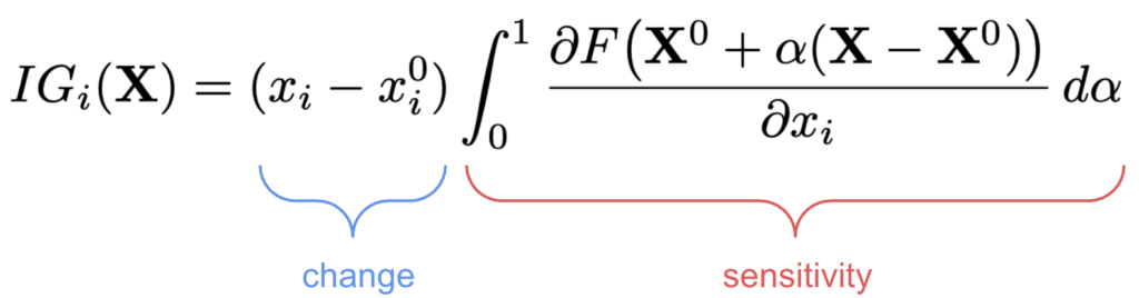
The formula we've spoken about up until now is actually only an approximation of IG. The true formula is given below. This is similar to before, except we are taking infinitesimal steps along the path from the baseline to input. This is the formula that satisfies the various axioms discussed in the paper.
\[
IG_i(\mathbf{X}) = (x_i - x_i^0) \int_{0}^{1}
\frac{\partial F\big(\mathbf{X}^0 + \alpha(\mathbf{X} - \mathbf{X}^0)\big)}{\partial x_i} \, d\alpha
\]
The problem is that this formula is impractical to apply as it would take far too long. This is why we take discrete steps. Thankfully, you will see when we apply the methods, after a certain number of steps, the method converges and we get a good approximation. The default with the Captum package is 50 steps.
Comparison to DeepLIFT
Talking about approximations, it has been shown that DeepLIFT provides an approximation of IG [1]. This was part of the work that showed you could calculate DeepLIFT using gradients. This was also demonstrated empirically by calculating the correlation of the attribution methods across multiple models. However, it does not work well for complex models with multiplicative components like Recurrent Neural Networks (RNNs).
You can see an example in Figure 2. In this case, we apply both IG and DeepLIFT to the same ResNet-18 model and image. You can see how we get similar saliency maps, but they are not exact. This may be good enough for your application, and considering that DeepLIFT only requires one backwards pass, it is often a better method in practice. We can obtain similar attributions but much faster.
Axioms
Much work has been done on the axioms of IG [2, 3, 4, 5, 6]. We discussed this in detail in the lesson on Axioms. Although we are still coming to a consensus on the exact properties, what is clear is that IG is likely the best method for computer vision problems from an axiomatic point of view. This becomes even more certain if we only consider gradient-based methods.
We make this conclusion as IG satisfies many axioms. In addition, methods that satisfy a similar number of axioms have issues when applied to computer vision problems. For example, baseline SHAP uses a baseline in a way that leads to out-of-distribution permutations. Similarly, kernelSHAP makes an assumption of feature independence, which is often unrealistic for image data.
Practically, this means we can be more certain that IG provides reliable saliency maps that reflect the true inner workings of the models. However, we must keep in mind that, although axioms can make these properties more likely, they do not guarantee them. In other words, we still need to apply the evaluation methods discussed in the lesson on Evaluation.
The interpretation of Integrated Gradients
To interpret IG, we can go back to the lesson on XAI Taxonomy. We introduce the definitions of sensitivity-based vs contribution-based attributions.
- Sensitivity-based attribution: how the output of the network changes for infinitesimally small perturbations around the original input.
- Contribution-based attribution: the marginal effect of a feature on the output with respect to a baseline.
It is argued that, for gradient-based methods, multiplying by the input changes them from a sensitivity-based to a contribution-based method [1]. However, we discussed how, for image data, this logic broke down for Input x Gradients. As this method only considers local gradients around the input, it assumes a linear relationship with the output. Additionally, unlike tabular features, pixel values do not have a clear causal relationship to the output. IG overcomes these limitations using a baseline.
With IG, the integral alone gives a measure of average sensitivity for each pixel along the path from the baseline to the input. This allows us to capture the non-linear relationships along that path. We then multiply this by the change in every pixel value. In other words, we get the contribution of each pixel by multiplying the change by how sensitive the model is to that change.
This provides a clear interpretation of IG, and it goes back to the importance of selecting a good baseline. We must be aware that IG saliency maps do not show absolute pixel importance. Instead, they show the contribution of each pixel to the difference in output between the original input and the baseline—this is the marginal effect. However, if the baseline produces a neutral prediction (e.g., a black or grey image with low confidence across all classes), then these marginal contributions could be interpreted as the importance for the final prediction. Ultimately, the choice of baseline fundamentally shapes what the attributions mean.
Applying Integrated Gradients with Captum
We move on to applying the method. We start with our imports. We will be importing the model from Hugging Face (line 7). We also have the Captum IG package (line 9). We will explore the attribution created using the default parameter for this function, as well as those created by varying the number of interpolation steps.
import matplotlib.pyplot as plt
import numpy as np

from PIL import Image

import torch
from transformers import AutoModelForImageClassification, AutoImageProcessor

from captum.attr import IntegratedGradients

# Helper functions
import sys
sys.path.append('../')

from utils.visualise import process_attributions
Load model
We will be applying IG to the same model as in the lesson on DeepLIFT. As a reminder, we load our model (lines 2-5) and wrap it so that it outputs logits (lines 8-16).
# Load model and processor
model_name = "hilmansw/resnet18-catdog-classifier"
base_model = AutoModelForImageClassification.from_pretrained(model_name)
processor = AutoImageProcessor.from_pretrained(model_name)
base_model.eval()

# Wrap model to return only logits
class WrappedModel(torch.nn.Module):
    def __init__(self, model):
        super().__init__()
        self.model = model
    def forward(self, x):
        outputs = self.model(x)
        return outputs.logits  # Captum needs a Tensor output

model = WrappedModel(base_model)
model.zero_grad()
The model is trained to classify images as either dogs or cats. We then load an example image and process it so it is ready for the model (lines 2-3).
# Load and preprocess images
dog_img = Image.open("dog.png") #Update path
dog_inputs = processor(images=dog_img, return_tensors="pt")
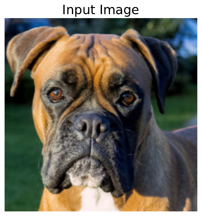
print(dog_inputs['pixel_values'].shape) # Should be [1, 3, 224, 224]As seen in Figure 3, this time we will be using the image of a dog. You can download this from Wikimedia Commons or use the code in the notebook.
We do a forward pass with this image (lines 2-4). The logits for the cat and dog classes are given by indices 0 and 1 in the output, respectively. Below, the output shows that we are predicting the correct class. Now, let's see how we can explain this prediction using IG.
# Forward pass
with torch.no_grad():
    logits = model(dog_inputs["pixel_values"])
    predicted_class_idx = logits.argmax(-1).item()

    print("Logits:", logits)
    print(f"Class idx: {predicted_class_idx}")
    print(f"Class:", base_model.config.id2label[predicted_class_idx])
Logits: tensor([[-5.7368, 8.0936]])
Class idx: 1
Class: dogsGenerating attributions
The process for obtaining attributions is also very similar to the one used in the DeepLIFT lesson. We start by creating an IntegratedGradients object by passing in our model (line 2).
# Initialize Integrated Gradients
model.zero_grad()
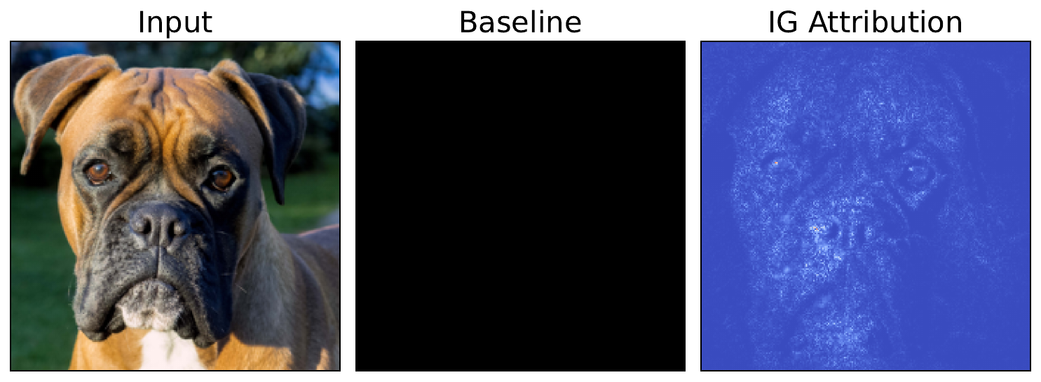
ig = IntegratedGradients(model)For this IG, we will only be using one baseline. We create a black baseline image (i.e. all zeros) (lines 2-3). We then pass this baseline (line 8), along with the input image (line 7) and target (line 9) to the IG object. This will output an attribution which you can see in Figure 4.
# Zero baseline
zero_baseline = np.zeros_like(dog_img)
zero_baseline_tensor = processor(images=zero_baseline, return_tensors="pt",crop_pct=1.0)

# Compute attributions
attributions = ig.attribute(
    inputs=dog_inputs["pixel_values"],
    baselines=zero_baseline_tensor["pixel_values"],
    target=1
)
When interpreting the attribution, we must remember that it provides the marginal contributions for each pixel. That is, it shows which pixels have contributed to the difference in the predicted logit from the dog class when we change the input from the baseline to the input image. It does not provide the absolute importance of each pixel.
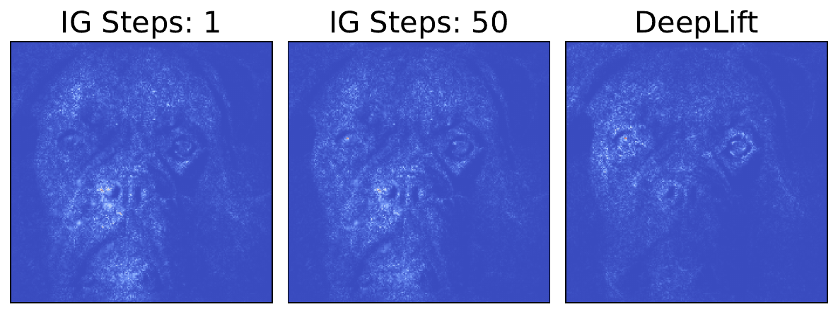
Varying the number of steps
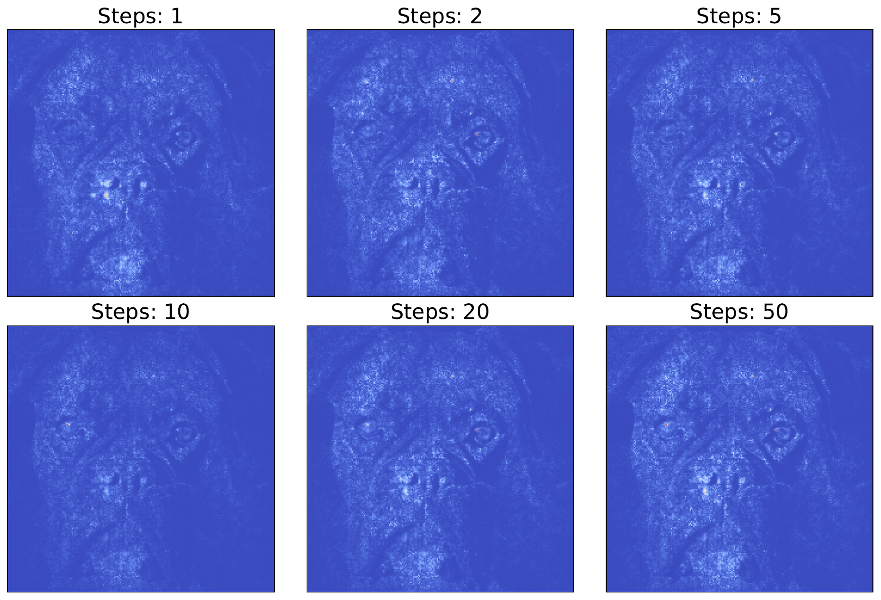
By default, the IG object will use 50 steps between the baseline and the input image to create the final attribution. We can vary this by changing the n_steps parameter (line 5). In Figure 5, you can see the output using a varying number of steps.
## Vary step number
attributions = ig.attribute(
    inputs=dog_inputs["pixel_values"],
    baselines=zero_baseline_tensor["pixel_values"],
    n_steps=10,
    target=1,
)
One thing to note is that the attributions are all visually quite similar. After a certain number of steps, they will converge, and the attribution will not change if you further increase them. This means that for some applications, it may make sense to reduce the number of steps. As each step requires an additional backwards pass, this can significantly reduce the computation time required.
The downside is that, if you reduce the number of steps, you will likely get a worse approximation of the integral formula we saw above. This means the resulting approximation will be less likely to satisfy all the axioms, leading to issues around reliability and faithfulness.
Again, as we discussed in the lesson on Axioms, these considerations depend on what you are trying to achieve. If you want to provide human-friendly explanations for model predictions, then you may want something that satisfies these axioms. If you only care about debugging a model, it may make more sense to use fewer steps or even choose one of the other gradient-based heuristic methods.
Challenge
Calculate the correlation between the IG saliency maps for step \(k\) and \(k-1\). Plot these for a given number of steps. What do you notice about the correlation values?
I hope you enjoyed this article! See the course page for more XAI courses. You can also find me on Bluesky | YouTube | Medium
Additional Resources
- YouTube Playlist: XAI for Tabular Data
- YouTube Playlist: SHAP with Python
Datasets
Conor O’Sullivan, & Soumyabrata Dev. (2024). The Landsat Irish Coastal Segmentation (LICS) Dataset. (CC BY 4.0) https://doi.org/10.5281/zenodo.13742222
Conor O’Sullivan (2024). Pot Plant Dataset. (CC BY 4.0) https://www.kaggle.com/datasets/conorsully1/pot-plants
Conor O'Sullivan (2024). Road Following Car. (CC BY 4.0). https://www.kaggle.com/datasets/conorsully1/road-following-car
References
- Ancona, Marco, Ceolini, Enea, \"Oztireli, Cengiz, et al. (2017). Towards better understanding of gradient-based attribution methods for deep neural networks. arXiv preprint arXiv:1711.06104.
- Sundararajan, Mukund, Taly, Ankur, Yan, Qiqi (2017). Axiomatic attribution for deep networks. International conference on machine learning, 3319--3328.
- Lundstrom, Daniel D, Huang, Tianjian, Razaviyayn, Meisam (2022). A rigorous study of integrated gradients method and extensions to internal neuron attributions. International Conference on Machine Learning, 14485--14508.
- Lerma, Miguel, Lucas, Mirtha (2021). Symmetry-preserving paths in integrated gradients. arXiv preprint arXiv:2103.13533.
- Sundararajan, Mukund, Najmi, Amir (2020). The many Shapley values for model explanation. International conference on machine learning, 9269--9278.
- Lundstrom, Daniel, Razaviyayn, Meisam (2025). Four axiomatic characterizations of the integrated gradients attribution method. Journal of Machine Learning Research, 26(177), 1--31.
Get the paid version of the course. This will give you access to the course eBook, certificate and all the videos ad free.