In deep learning, gradients are typically used to train a model. They update parameters and ultimately form the complex features used to make predictions. When it comes to XAI, gradients are used to reveal those same features. The most basic approach is to look at the raw gradients of a network [1]. These are known as Vanilla Gradients.
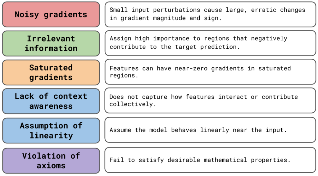
In practice, this approach is rarely used. The more popular and reliable gradient-based methods will all alter raw gradients in some way. To understand why, we are going to focus on the limitations of vanilla gradients. You can see these in Figure 1.
To demonstrate these limitations, we will use Python to visualise vanilla gradients. This will give you the necessary skills and knowledge to apply other gradient-based methods. In the later sections, we will see how these other methods build on vanilla gradients to address its limitations.
Before you get stuck into the article, here is the video version of the lesson. Note: Some updates have been made to the article after the video was posted. Specifically, we have added sections on the assumption of local linearity and the violation of axioms. We also combined the discussion of unstable gradients and rapid sign changes under a single “Noisy Gradients” heading.
How vanilla gradients are calculated
Vanilla gradients are the gradients of the output w.r.t. the input image. All we need to obtain these is backpropagation. Typically, backpropagation is used to calculate gradients that are then used to update the parameters of a network. This is also usually done with a batch of images. Vanilla gradients use backpropagation in a different way. That is, using an individual input image, we find the gradients of the loss (\(L\)) w.r.t. the pixels in the image (\(X\)):
\[
\frac{\partial L}{\partial X}
\]
This is also called a derivative or rate of change. Intuitively, pixels that have large gradients (both positive and negative) have a large impact on the loss. In other words, they are more important to the prediction for a given image. By visualising all gradients, we can create a saliency map showing important regions in the image.
For classification problems, we are usually interested in the predicted class (\(y_c\)). That is the one with the highest logit. So, when calculating vanilla gradients, we will instead take gradients of the output logit for this class (\(y_c\)) w.r.t. the input image (\(X\)). These will tell us how important the pixels are to the predicted class and not all logits in general.
\[
\frac{\partial y_c}{\partial X}
\]
To start the backwards pass from this logit, we set \(\frac{\partial L}{\partial y_c} = 1 \) and all \(\frac{\partial L}{\partial y_j} = 0 \). This is the same as saying that the score for this class is 1, and all other classes have a score of 0. The backpropagation process is then the same as before.
\[
\frac{\partial L}{\partial X} = \frac{\partial L}{\partial y_c}\frac{\partial y_c}{\partial X} + \sum_{j \neq c } \frac{\partial L}{\partial y_j}\frac{\partial y_j}{\partial X} = \frac{\partial y_c}{\partial X}
\]
The interpretation of gradients for visualisation
We've touched on it already but it is important to clarify the interpretation of gradients. Using permutation-based methods in the previous section, we could make claims like "a region of pixels has increased the prediction". We need to be careful when making these same claims using gradients. When interpreting gradients w.r.t. input pixels, it is best to focus on their magnitude rather than their sign.
This may be confusing when we consider how gradients are normally used. When doing backwards propagation, a positive gradient indicates that we should decrease a parameter to decrease the loss. When looking at the gradients of a logit, this interpretation switches. A positive gradient indicates that we should increase the value of the parameter to increase the value of the logit. In other words, we can say a positive movement in the parameter supports the prediction. However, when looking at gradients of input pixels, it is no longer clear which direction should be associated with supporting or opposing the prediction.
For example, take a model that classifies images of dogs and cats. Looking at Figure 2, suppose the pixels on a dog's nose have a positive gradient. This suggests that increasing the pixel values, making them slightly lighter in colour, would increase the dog logit. However, if the gradients were negative, we could similarly increase the logit by decreasing the pixel values, making them slightly darker in colour. Why should one colour change be associated with supporting the prediction and not the other?
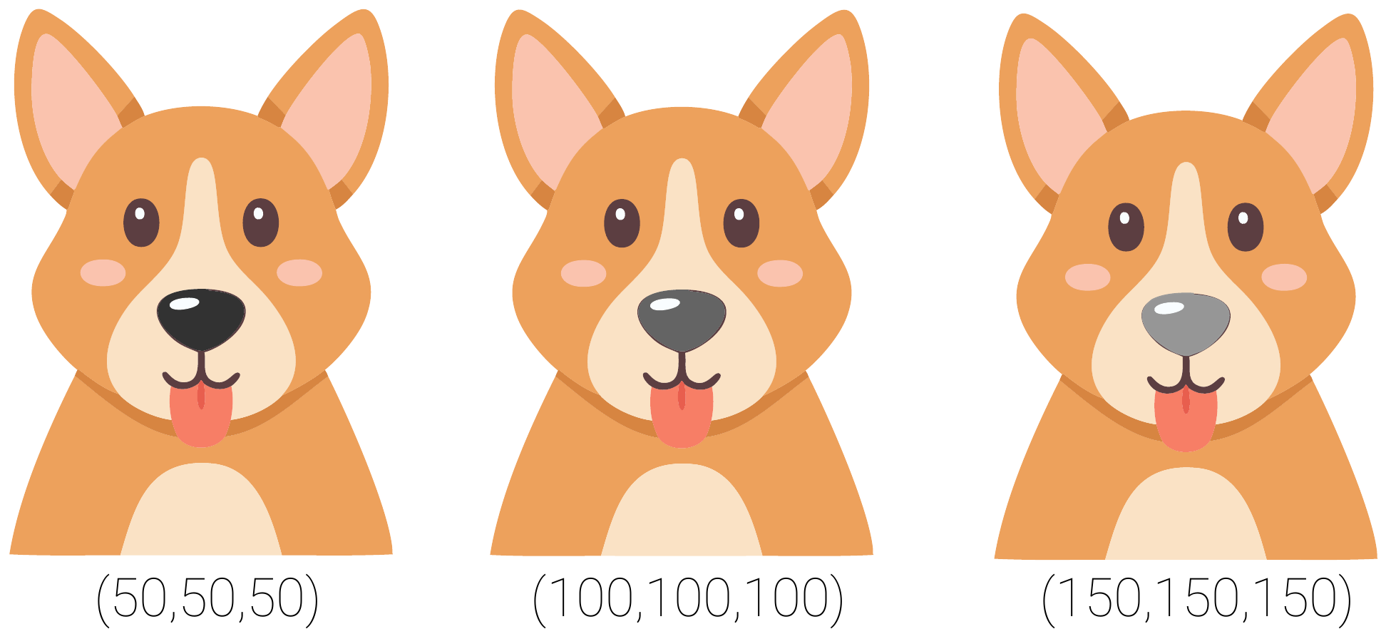
In short, the direction in which we change an input pixel has no inherent causal interpretation. Although we could say that a movement in a pixel supports or opposes a prediction, this does not mean we can say that the pixel supports or opposes a prediction. Ultimately, we can not tell how a pixel has influenced a prediction, only that it is important.
The limitations of vanilla gradients
This interpretation of gradients is one of their important weaknesses. It limits the conclusions we can make using vanilla gradients. Ultimately, both positive and negative gradients are an indication that a pixel is important, and we should stick to interpreting their magnitude. However, as we will discuss, even sticking to the magnitude has its problems — something that other gradient-based methods aim to address.
Noisy Gradients
The biggest problem is that gradients can be extremely sensitive to small changes in the input. Small movements in pixel values can lead to large changes in magnitude and even flip the sign of a gradient. This can lead to saliency maps that are hard to interpret, as they will seem random or speckled, even in regions that should be smooth or semantically meaningful. You can see this in Figure 3. The speckled image on the right shows how the sign changes even for neighbouring pixels with similar colours and textures.
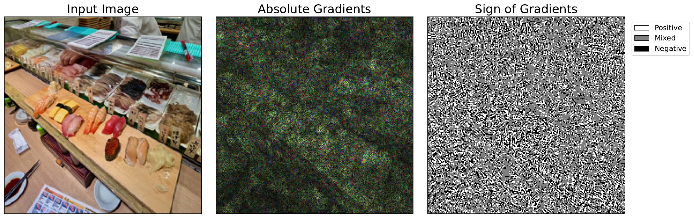
A major cause is the non-linearity of neural networks. Activation functions like ReLU create sharp boundaries where gradients abruptly switch from zero to non-zero. When a neuron's value crosses one of these thresholds, its gradient can change drastically. Complex interactions between layers can also mean that gradients can behave unpredictably. For the case of sign flipping, this is why we often take the absolute value of vanilla gradients.
A method called SmoothGrad has also been shown to help [2]. The paper's subtitle sums it up — adding noise to remove noise. It works by creating augmentations of the input image by artificially adding noise. Then, we take the average gradient across all augmentations. This helps reveal more consistent patterns. Keep in mind, that this method can be used with any gradient-based methods and not only vanilla gradients.
Irrelevant information
Another factor that leads to noisy saliency maps is that gradients often contain information that is not specific to the target logit. Often, we only want to understand the regions or features that support a prediction. However, gradients can be large in regions that negatively contribute to the predicted logit. These can come from background pixels or features associated with other classes.
Guided backpropagation can clean up saliency maps with a technique called ReLU masking. This alters the ReLU activation functions of a network so they suppress negative gradients during backpropagation. The result is a visually sharper saliency map that highlights the features used by a model. However, this method is not class-discriminative, meaning it may still highlight features useful for multiple classes, not just the target one.
Grad-CAM is a more reliable class-discriminative method. It aggregates activated feature maps in the last convolutional layer of a network. When doing this, it weights the feature maps using the average gradient of their elements. By focusing on deeper layers, where features are more semantically meaningful, Grad-CAM better identifies regions that support a specific prediction. We discuss this in more depth in the lesson on Guided Grad-CAM.
Saturated Gradients
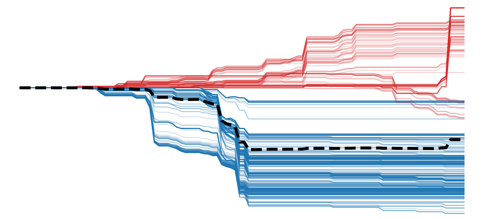
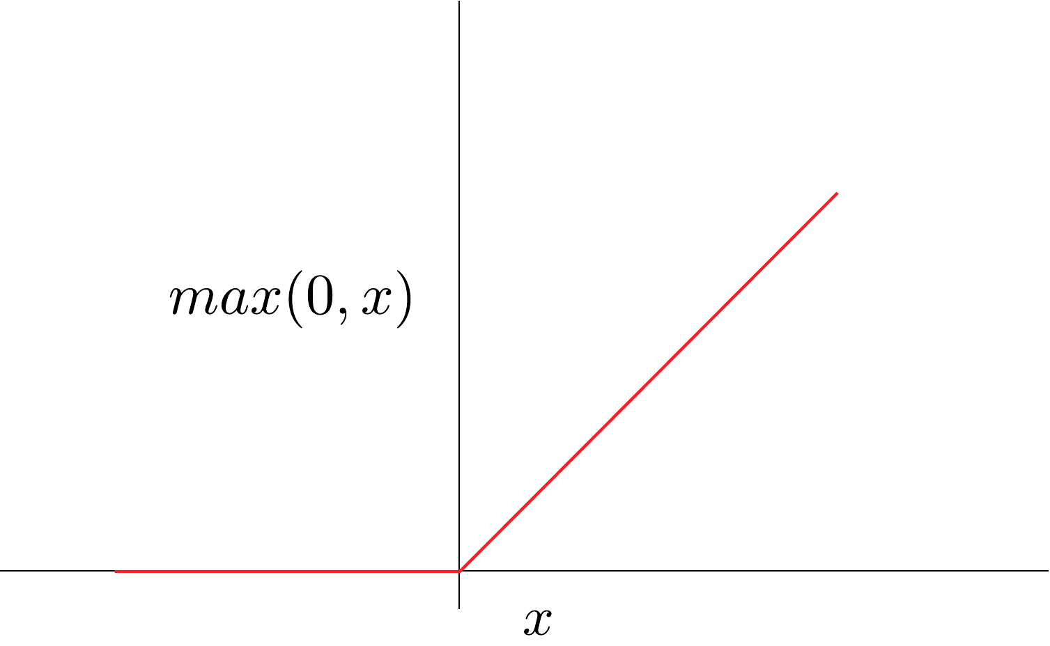
In some cases, the gradients of important pixels can be small or even zero. Take the ReLU activation function in Figure 4. During backpropagation, if the input to the function is a negative value, then the gradients will be zero — regardless of how large the negative input is. This is true even for very large negative values, which is an indication that the input is important to the prediction. This can lead to regions in the input where the gradients become flat, giving us a saliency map that suggests they are not important.
Integrated Gradients (IG) overcomes this problem using a baseline image. This is an uninformative, usually all-black image. This method takes an average of gradients computed along a straight-line path from the baseline input to the actual input. This avoids the saturation problem as we do not observe gradients at a single point. Instead, we can see how they change over the path.
Vanishing gradients is a similar problem. In large networks, during training, the gradients of earlier layers can become extremely small or even zero. This is because they are obtained by iteratively multiplying the gradients from deeper layers, which are all small numbers themselves. By the time we get to the image, the gradients may indicate that a pixel is not important, even though it is used in the deeper layers.
Thankfully, this problem has largely been solved by changes to model architecture. Using mechanisms like residual connections and normalisation, we can avoid vanishing gradients in training and subsequently in our interpretations. Although it is worth mentioning that Grad-CAM would not be impacted by this problem. This is because it uses the gradients from deeper convolutional layers.
Lack of Context Awareness
Another problem is that vanilla gradients reflect local sensitivity. That is how much a small change in an input pixel would change the output. This does not capture how specific features or regions in the image contribute to a prediction. Due to interactions, the effect of changing multiple pixels simultaneously differs from the sum of their individual effects.
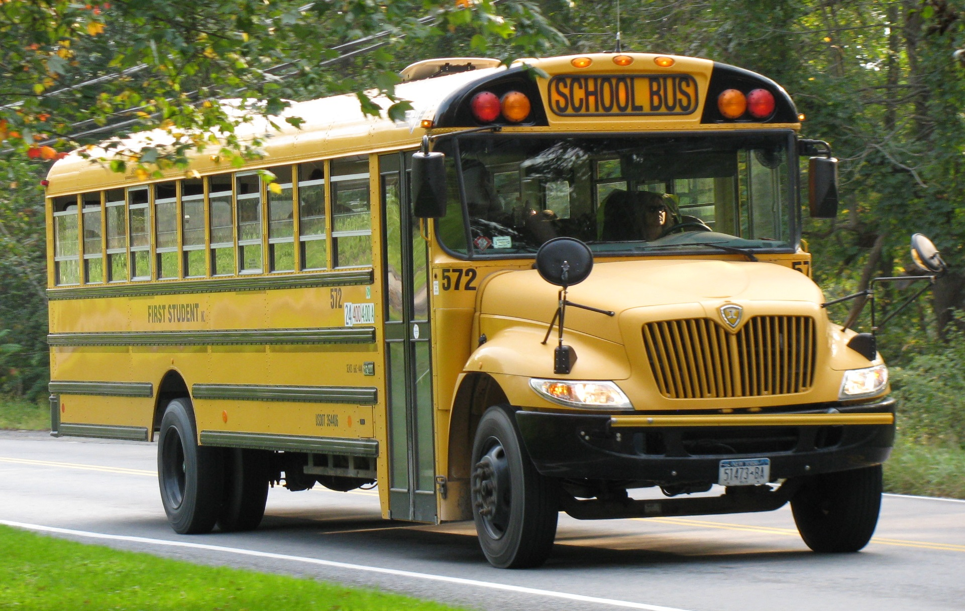
Consider the image of a school bus in Figure 5. A model may be able to classify this correctly, but it is unlikely to rely on an individual pixel to do this. Likely, a yellow pixel in the context of many other yellow pixels has increased the school bus logit. Both the presence of wheels and the yellow body could increase the score. Even the presence of the road under the bus might have contributed. It is all these aspects contributing together that lead to our final prediction. Ultimately, the non-linear nature of deep learning models means we can miss important details when looking at changes in individual pixels.
Grad-CAM can partially address this issue as it uses the gradients from deeper layers of the network. As we progress through the layers of a CNN, we go from simple features like edges and textures to more complex ones like object parts, then entire objects. So, the elements of these deeper layers contain detailed semantic information. In other words, they can capture interactions between objects or regions in an image.
Assumption of local linearity
A related problem is that vanilla gradients assume the model's behaviour is locally linear around the input. That is, we are assuming that if we change the pixel, then the target will change proportionally to the gradient. However, as we discussed above, neural networks are highly non-linear. This means gradients may not accurately represent how the model behaves over meaningful input variations.
IG can help mitigate the previous two problems. This is because the method changes all pixels simultaneously along a path from the baseline to the input image. For the prior limitation, the simultaneous changes can capture how features interact. For the latter, the path allows us to understand the changes in gradients over meaningful changes to the input. IG is also more sound from an axiomatic point of view.
Does not satisfy axioms
We discussed various desirable mathematical properties in the lesson on Axioms. Vanilla gradients will not satisfy any of them consistently. For example, the sum of all gradients cannot account for the entire prediction (i.e. completeness). As we discussed, even basic axioms like dummy won't be satisfied, as features that don't actually affect the model's output can still have non-zero gradients due to saturation or local noise. This can lead to reliability and faithfulness issues down the line.
Vanilla gradients with Python
With all these limitations, it is still worth applying the method. As we will see, the code will provide a valuable building block for more complex methods. We start with our imports.
import matplotlib.pyplot as plt
import matplotlib.patches as mpatches
import numpy as np

from PIL import Image

import torch
from torchvision import models

# Helper functions
import sys
sys.path.append('../')

from utils.visualise import display_imagenet_output, process_attributions
from utils.datasets import preprocess_imagenet_image
Load model and input image
For our model, we'll use VGG16 pretrained on ImageNet. To help, we have the two functions below. These will also be used later in the course throughout the gradients-based section. We already explained these in the lesson on LIME but let's repeat that in case you skipped that section.
The first function, preprocess_imagenet_image, will correctly format an image for input to the model. The normalisation values used are the mean and standard deviation of the images in ImageNet. The code for this function is found in the dataset.py file in the utils folder.
def preprocess_imagenet_image(img_path):

    """Load and preprocess images for PyTorch models."""

    img = Image.open(img_path).convert("RGB")

    #Transforms used by imagenet models
    transform = transforms.Compose([
        transforms.Resize((224, 224)),
        transforms.ToTensor(),
        transforms.Normalize(mean=[0.485, 0.456, 0.406], std=[0.229, 0.224, 0.225]),
    ])

    return transform(img).unsqueeze(0)
ImageNet has many classes. The second function, display_imagenet_output will format the output of the model to display the classes with the highest predicted probabilities. This can be found in the visualise.py file in the utils folder.
def display_imagenet_output(output,n=5):

    """Display the top n categories predicted by the model."""

    # Download the categories
    url = "https://raw.githubusercontent.com/pytorch/hub/master/imagenet_classes.txt"
    urllib.request.urlretrieve(url, "imagenet_classes.txt")

    with open("imagenet_classes.txt", "r") as f:
        categories = [s.strip() for s in f.readlines()]

    # Show top categories per image
    probabilities = torch.nn.functional.softmax(output[0], dim=0)
    top_prob, top_catid = torch.topk(probabilities, n)

    for i in range(top_prob.size(0)):
        print(categories[top_catid[i]], top_prob[i].item())

    return top_catid[0]
We load the pretrained VGG16 model (line 2), move it to a GPU (lines 5-8) and set it to evaluation mode (line 11). You can see a snippet of the model output below. These show 5 of 13 convolutional layers. There are also 3 fully connected layers that make up the 16 weighted layers in VGG16.
# Load the pre-trained model (e.g., VGG16)
model = models.vgg16(pretrained=True)

# Set the model to gpu
device = torch.device('mps' if torch.backends.mps.is_built()
                      else 'cuda' if torch.cuda.is_available()
                      else 'cpu')
model.to(device)

# Set the model to evaluation mode
model.eval()
model.zero_grad()
VGG(
(features): Sequential(
(0): Conv2d(3, 64, kernel_size=(3, 3), stride=(1, 1), padding=(1, 1))
(1): ReLU(inplace=True)
(2): Conv2d(64, 64, kernel_size=(3, 3), stride=(1, 1), padding=(1, 1))
(3): ReLU(inplace=True)
(4): MaxPool2d(kernel_size=2, stride=2, padding=0, dilation=1, ceil_mode=False)
(5): Conv2d(64, 128, kernel_size=(3, 3), stride=(1, 1), padding=(1, 1))
(6): ReLU(inplace=True)
(7): Conv2d(128, 128, kernel_size=(3, 3), stride=(1, 1), padding=(1, 1))
(8): ReLU(inplace=True)
(9): MaxPool2d(kernel_size=2, stride=2, padding=0, dilation=1, ceil_mode=False)
(10): Conv2d(128, 256, kernel_size=(3, 3), stride=(1, 1), padding=(1, 1))
.
.
.We display our example image (Sushi image: commons.wikimedia.org/wiki/File:Sushi_japan.png) that will be used as input into the model (lines 2-6). You can see this in Figure 6. I took this on a recent trip to Japan. ImageNet has no class for sushi so it will be interesting to see what prediction it makes.
# Load a sample image
img_path = "sushi.png"
img = Image.open(img_path).convert("RGB")

plt.imshow(img)
plt.title("Input")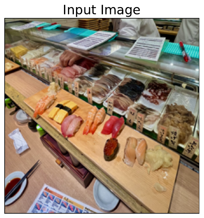
You can download the example image directly from Wikimedia Commons using the URL below (line 3). Alternatively, as seen below, you can use the save_image function from the download.py file in the utils folder. Similar code will be available for any lesson that uses this image source.
from utils.download import save_image

url = "https://upload.wikimedia.org/wikipedia/commons/a/ae/Sushi_japan.png"
save_image(url, "sushi.png")
Let's get a prediction for this image and visualise its gradients using standard backpropagation. These are our vanilla gradients. In the next section, we will compare these to gradients obtained using Guided Backpropagation.
Standard backpropagation
We start by processing our image (line 2) and moving it to a GPU (line 3). The tensor gradients are stored and can be accumulated or overridden. So, to avoid doing this unintentionally, it is good practice to clone the input tensor (line 6). Usually, gradients are not calculated for the input image as they are only used to update model parameters. This means we must also enable gradient tracking for the image tensor (line 7).
# Preprocess the image
original_img_tensor = preprocess_imagenet_image(img_path)
original_img_tensor = original_img_tensor.to(device)

# Clone tensor to avoid in-place operations
img_tensor = original_img_tensor.clone()
img_tensor.requires_grad_() # Enable gradient tracking
We now do a forward pass to get a prediction for the input image (line 1). We then display the output (line 4). Below, you can see the top 5 predictions. Given all the possible classes, a grocery store seems like a reasonable prediction.
predictions = model(img_tensor)

# Decode the output
display_imagenet_output(predictions,n=5)
grocery store 0.2256142646074295
tobacco shop 0.21862675249576569
confectionery 0.17332792282104492
bakery 0.10615035146474838
hotdog 0.04379023611545563Before we do a backwards pass, it is good practice to reset the model's gradients (line 2). Again, this is because gradients can be accumulated when making multiple backwards passes. We want to find the gradients of the logit with the highest score. We select this (line 5) and use it to perform a backwards pass (line 8). This will calculate the gradients of this logit w.r.t. activations of intermediate layers and input values.
# Reset gradients
model.zero_grad()

# Select the class with the highest score
target_class = predictions.argmax()

# Compute gradients w.r.t to logit by performing backward pass
predictions[:, target_class].backward()
The backwards pass will update img_tensor with the gradients. This allows us to select the gradients from the tensor (line 2). We also detach the gradients so that any operations do not impact the original tensor (line 2). Outputting the shape gives us dimensions (1, 3, 244, 244). We have a batch size of 1 and gradients for the 3 RGB channels in our input image. These results give us \((\frac{\partial y_c}{\partial X})\) or, in other words, how a small change in each input pixel would affect the target logit.
# Get the gradients
standard_backprop_grads = img_tensor.grad.detach().cpu().numpy()
print(standard_backprop_grads.shape) # (1, 3, 224, 224)
We'll use the process_attributions function to help visualise the gradients. It gives a few options. It is common to take the absolute value of gradients when visualising vanilla gradients. This has to do with the interpretation of gradients we discussed earlier.
def process_attributions(
raw_attributions: torch.Tensor,
activation: str | None = None, # ['abs', 'relu', 'none']
normalize: bool = True,
skew: float = 1.0,
grayscale: bool = False,
colormap: str | None = None, # <– Default: None (no colormap)
output_as_pil: bool = False
):
"""
Visualize gradient or attribution maps for image classification.
Args:
attribution (torch.Tensor): Attribution map with shape (C, H, W) or (H, W).
activation (str): Activation applied to attributions ('abs', 'relu', or 'none').
normalize (bool): Whether to normalize attributions to [0, 1].
skew (float): Exponent to skew intensities (gamma correction). Only valid if normalize=True.
grayscale (bool): If True, converts output to grayscale before applying colormap.
colormap (str or None): Matplotlib colormap ('hot', 'coolwarm', etc.) or None for no color mapping.
output_as_pil (bool): If True, returns a PIL Image instead of NumPy array.
Returns:
np.ndarray or PIL.Image: Visualized attribution map (RGB or grayscale).
"""
# — Safety checks —
if not normalize and skew != 1.0:
raise ValueError("Cannot apply skew without normalization. Set normalize=True or skew=1.0.")
if activation not in ["abs", "relu", None]:
raise ValueError("Invalid activation. Choose from ['abs', 'relu', None].")
if grayscale and colormap is not None:
warnings.warn("Grayscale=True overrides colormap choice. Colormap will be ignored.", UserWarning)
# Convert to NumPy
if isinstance(raw_attributions, torch.Tensor):
attribution = raw_attributions.detach().cpu().numpy()
else:
attribution = raw_attributions.copy()
# Handle multi-channel case (1, C, H, W)
if attribution.shape[0] == 1:
attribution = attribution[0]
if attribution.ndim == 3 and attribution.shape[0] == 3:
attribution = np.transpose(attribution, (1, 2, 0)) # C, H, W -> H, W, C
# — Apply activation —
if activation == "abs":
attribution = np.abs(attribution)
elif activation == "relu":
attribution = np.maximum(0, attribution)
# 'none' -> do nothing
# — Normalization —
if normalize:
attribution -= attribution.min()
if attribution.max() > 0:
attribution /= attribution.max()
# — Skewing (gamma correction) —
if skew != 1.0:
attribution = np.power(attribution, skew)
# — Visualization logic —
if grayscale or (colormap is not None):
# Return single-channel map (grayscale look)
if attribution.ndim == 3:
attribution = np.mean(attribution, axis=-1)
attribution_img = np.uint8(255 * np.clip(attribution, 0, 1))
result = cv2.cvtColor(attribution_img, cv2.COLOR_GRAY2RGB)
if colormap is not None:
cmap = cm.get_cmap(colormap)
colored = cmap(attribution)[:, :, :3]
result = np.uint8(255 * colored)
else:
# No colormap, return as RGB
result = attribution
if output_as_pil:
return Image.fromarray(result)
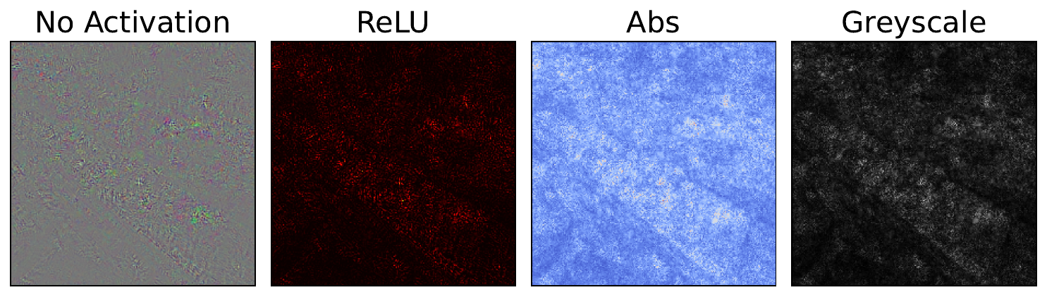
return resultWe use this function to display our gradients in a few different ways. You can see these in Figure 7. In each case, the gradients are normalised and skewed. The latter operation means that smaller gradients are given more weight in the visualisation. This reduces the impact of larger outlier gradients.
standard_grads = standard_backprop_grads[0].copy()

# Process the gradients
raw_grads = process_attributions(standard_grads, normalize=False)
print(raw_grads.shape) # (224, 224, 3)
print(np.min(raw_grads), np.max(raw_grads)) #-0.13959521 0.15818407

# Different visualisation variants
no_activation_grads = process_attributions(standard_grads)
relu_grads = process_attributions(standard_grads, activation="relu",  colormap="hot")
abs_grads = process_attributions(standard_grads, activation="abs",skew= 0.5, colormap="coolwarm")
grey_grads = process_attributions(standard_grads, activation="abs",skew= 0.8, grayscale=True)
With vanilla gradients, you can already see some important regions. It looks like the table and glass are contributing to the prediction. However, there is a lot of noise in the output. Potentially, all of the limitations we discussed are contributing to this. However, the issues around noisy gradients are the most likely culprits.
In the next section, we will discuss another simple approach — Input x Gradients. We will see that, although multiplying by the input pixel does provide clearer visualisations, the interpretations of the resulting saliency maps are a bit dubious. Later, we will apply Guided Backpropagation, which has a more intuitive interpretation. Both of those sections start where we leave off here. That is, we use the same imports, model and example image.
Challenge
Apply the code to a different input image. Does the saliency map make sense?
I hope you enjoyed this article! See the course page for more XAI courses. You can also find me on Bluesky | YouTube | Medium
Additional Resources
- YouTube Playlist: XAI for Tabular Data
Datasets
Conor O’Sullivan, & Soumyabrata Dev. (2024). The Landsat Irish Coastal Segmentation (LICS) Dataset. (CC BY 4.0) https://doi.org/10.5281/zenodo.13742222
Conor O’Sullivan (2024). Pot Plant Dataset. (CC BY 4.0) https://www.kaggle.com/datasets/conorsully1/pot-plants
Conor O'Sullivan (2024). Road Following Car. (CC BY 4.0). https://www.kaggle.com/datasets/conorsully1/road-following-car
References
- Simonyan, Karen, Vedaldi, Andrea, Zisserman, Andrew (2013). Deep inside convolutional networks: Visualising image classification models and saliency maps. arXiv preprint arXiv:1312.6034.
- Smilkov, Daniel, Thorat, Nikhil, Kim, Been, et al. (2017). Smoothgrad: removing noise by adding noise. arXiv preprint arXiv:1706.03825.
Get the paid version of the course. This will give you access to the course eBook, certificate and all the videos ad free.