Guided Grad-CAM
How to combine Guided Backpropagation and Grad-CAM for fine-grained, class-discriminative saliency maps

Why Grad-CAM and Guided Backpropagation complement each other

In the context of XAI, we say an explanation is class discriminative if it only reveals the features or locations in an image that are important for a given class. So, given an image that contains two objects, we would be able to isolate the features from only one of the objects. One way to assess this property is using the visualisation in Figure 1. We discussed this in the evaluation lesson. We can see that, compared to the other saliency maps, GBP struggles to identify features that can distinguish the dog class from the cat class.

At first, it may be surprising that GBP is not class-discriminative. Looking at Figure 2, we can see examples of feature maps extracted at different layers of a CNN. Earlier layers may extract certain features like edges and textures from the input. These are then combined in deeper layers to create features representing specific objects, like pieces of sushi. When applying GBP, we discussed how it reveals these features by only propagating gradients that contribute positively to a prediction. Specifically, we are propagating the gradients of the target logit w.r.t. the input \( ( \frac{\partial y_c}{\partial X} )\). So, as we are using the gradients of the target logit, should we not only see features that have contributed to that class?

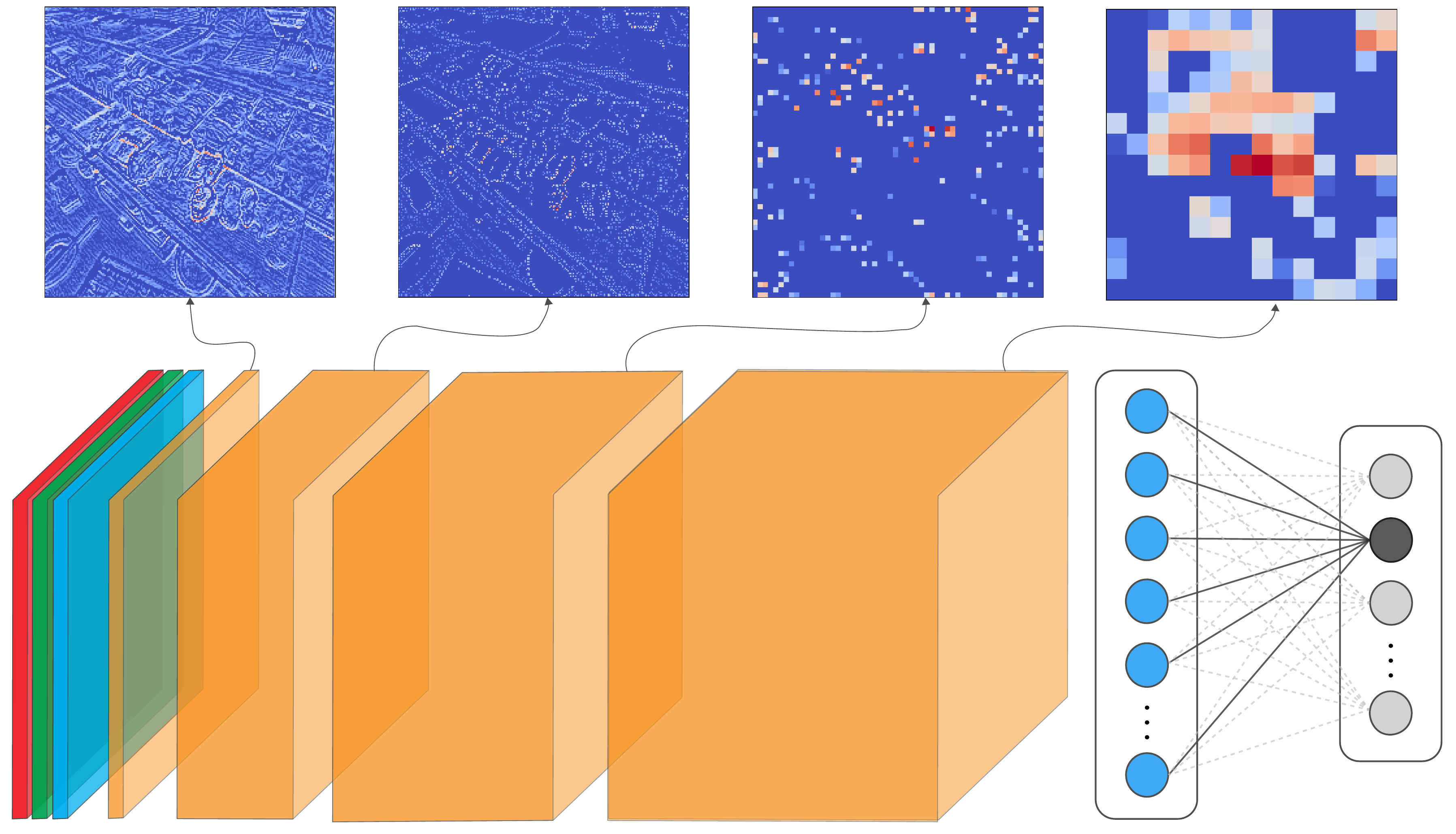
To be specific, with GBP, we are propagating the gradients from one layer that have contributed positively to the next layer in the network. The problem is that a feature map in an earlier layer can contain similar features, like edges and textures. So, we could have a situation where an edge detector might contribute positively to a deeper layer's feature map, even if that edge comes from an irrelevant region of the image. Even earlier feature maps could then contribute positively to the edge detector and so on. In other words, due to the hierarchical nature of the features extracted by the network, the class-discriminative nature of the gradients is dispersed as they are propagated backwards.

Now, going back to the lesson on Grad-CAM, we saw that method worked by combining all the feature maps in a convolutional layer. It also did this using gradients of the target logit. The difference is that Grad-CAM usually focuses on the final convolutional layer in the network. These are close to the output and will contain rich semantic and spatial information. As a result, gradients will be strongest in the spatial locations of the objects that have contributed positively to the target logit. The downside, as we have seen, is that these deep layers have a lower resolution.

Thankfully, by combining the attributes of both methods, we mitigate both of their limitations. We do this using element-wise multiplication of the individual saliency maps. In the end, GBP is used to find all detailed features, and Grad-CAM shows the locations of the important ones. Let's see how this is done in practice.

Applying Guided Grad-CAM with Captum

We start with our imports. These are similar to the previous lessons. The main difference is that we will now use the Captum package (line 9). We'll be using it to apply Guided Grad-CAM as well as GBP and Grad-CAM. So this section also provides some alternative code for the latter two methods.

import matplotlib.pyplot as plt
import numpy as np

from PIL import Image

import torch
from torchvision import models

from captum.attr import GuidedGradCam, GuidedBackprop, LayerGradCam

# Helper functions
import sys
sys.path.append('../')

from utils.visualise import display_imagenet_output, process_grads
from utils.datasets import preprocess_imagenet_image

Load model and image

We're going to use the same sample image and model as in the GBP lesson. We won't go into detail again, but as a reminder we are using the VGG16 architecture pretrained on ImageNet. For Guided Grad-CAM, we are particularly interested in the features.29 layer as it is the last convolutional layer of the network. Below you can see how we load the image, the model and get a prediction on the image.

# Load a sample image
img_path = "sushi.png"
img = Image.open(img_path).convert("RGB")

# Load the pre-trained model (e.g., VGG16)
model = models.vgg16(pretrained=True)

# Set the model to gpu
device = torch.device('mps' if torch.backends.mps.is_built() 
                      else 'cuda' if torch.cuda.is_available() 
                      else 'cpu')
model.to(device)

# Set the model to evaluation mode
model.eval()
model.zero_grad()

# Preprocess the image
original_img_tensor = preprocess_imagenet_image(img_path)
original_img_tensor = original_img_tensor.to(device)

# Clone tensor to avoid in-place operations
img_tensor = original_img_tensor.clone()
img_tensor.requires_grad_() # Enable gradient tracking

with torch.no_grad():
    predictions = model(img_tensor)

# Decode the output
display_imagenet_output(predictions,n=5)

Guided Grad-CAM attributions

To get the Guided Grad-CAM attribution, we start by selecting the last convolutional layer as our target layer (line 2). We also selected a target class (line 3). This is the class with the highest predicted logit for the input image. In this case, it is class 582 of ImageNet, which has the label 'grocery store, grocery, food market, market'.

# Specify the target layer and class
target_layer = model.features[29]  # last conv layer in VGG16
target_class = torch.argmax(predictions, dim=1).item()

Using the model and target layer, we initialise the Guided Grad-CAM object (line 2). We then pass our image tensor and target class to this object to get an attribution (lines 3-4).

# Get attributions
ggc = GuidedGradCam(model, target_layer)
ggc_attr = ggc.attribute(img_tensor, 
                        target=target_class)

We then process the attribution (line 2) and display it as before. You can see the output in Figure 3. For this, it is clear that the features from the food items are likely leading to the grocery store/food market prediction.

# Process for visualization
ggc_attr = process_attributions(ggc_attr)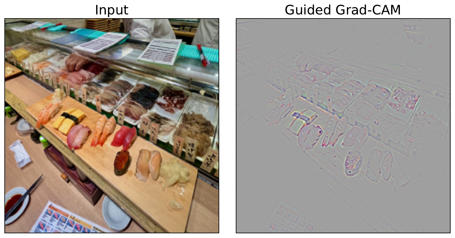

Grad-CAM and Guided Backpropagation attributions

Guided Grad-CAM is simply a combination of Guided Backpropagation and Grad-CAM. As mentioned, the former provides information about detailed features from earlier layers and the latter provides class-discriminative information from deeper layers. To see this, let's apply both of these methods using Captum.

We start with the Grad-CAM object (line 2). Like with the Guided Grad-CAM, we must pass both the model and the target layer. We then get the Grad-CAM attribution (line 3) and process it. This involves upsampling to the dimensions of the input image (lines 6-8) and formatting it as a Numpy array (line 9).

# Grad-CAM
layer_gc = LayerGradCam(model, target_layer)
gc_attr = layer_gc.attribute(img_tensor, target=target_class)

# Process and upsample
gc_attr_upsampled = torch.nn.functional.interpolate(
    gc_attr, size=(224, 224), mode='bilinear', align_corners=False
)[0][0]
gc_attr_np = gc_attr_upsampled.cpu().detach().numpy()

We then follow a similar process for the GBP attributions. In this case, we do not need to pass the target layer (line 2) as this method will propagate gradients all the way back to the input pixels.

# Guided Backprop
guided_bp = GuidedBackprop(model)
gb_attr = guided_bp.attribute(img_tensor, target=target_class)

gb_attr = process_attributions(gb_attr)

Finally, we visualise all three of our attributions (lines 2-11). For Grad-CAM, we have overlaid the attribution on the original image (lines 3-5). In Figure 4, you can see how the Guided Grad-CAM attribution is a combination of the other two. The result is an emphasis on the detailed features contributing to the prediction.

# Visualize
fig, ax = plt.subplots(1,3, figsize=(15,5))
ax[0].imshow(img)
ax[0].imshow(gc_attr_np, cmap='jet', alpha=0.5)
ax[0].set_title("Grad-CAM")

ax[1].imshow(gb_attr, cmap='jet')
ax[1].set_title("Guided Backpropagation")

ax[2].imshow(ggc_attr)
ax[2].set_title("Guided Grad-CAM")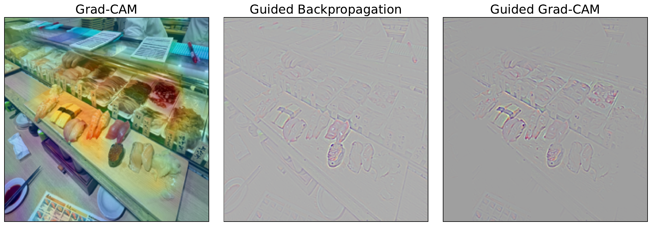

As we have seen, both Grad-CAM and Guided Backpropagation have their limitations. When we combine them, we can mitigate the limitations to a certain extent. However, we must keep in mind that they are both still based on simple heuristics. They are not based on any mathematical theory and will likely violate most axioms. As a result, they can produce misleading attributions.

The next methods we will discuss attempt to provide better saliency maps. SmoothGrad improves reliability by reducing the impact of noisy gradients. On the other hand, DeepLIFT and more so Integrated Gradients seek to improve faithfulness by providing axiom-based explanation methods.

Challenge

Apply the test of discriminativity visualisation to both GBP and Guided Grad-CAM. Use an image where objects from two ImageNet classes are present, like in Figure 1.

References

- Smilkov, Daniel, Thorat, Nikhil, Kim, Been, et al. (2017). Smoothgrad: removing noise by adding noise. arXiv preprint arXiv:1706.03825.
Get the paid version of the course. This will give you access to the course eBook, certificate and all the videos ad free.